Numerical Methods for Stiff ODEs and Differential-Algebraic Equations

Before jumping into this lecture, I want to start by mentioning that DAEs are not ODEs. There are substantial differences that must be addressed. The abstract is rather clear:

This paper outlines a number of difficulties which can arise when numerical methods are used to solve systems of differential/algebraic equations of the form. Problems which can be written in this general form include standard ODE systems as well as problems which are substantially different from standard ODE’S. Some of the differential/algebraic systems can be solved using numerical methods which are commonly used for solving stiff systems of ordinary differential equations. Other problems can be solved using codes based on the stiff methods, but only after extensive modifications to the error estimates and other strategies in the code. A further class of problems cannot be solved at all with such codes, because changing the stepsize causes large errors in the solution. We describe in detail the causes of these difficulties and indicate solutions in some cases.

However, a good portion of those issues can be mitigated by symbolic tooling which will be covered in later lectures. Other aspects will be highlighted on an as-needed basis. If you want more details, refer to that classic article.

That said, we will be using stiff ODEs to introduce the numerical methods for DAEs since, while they are distinctly not the same, many of the methods for DAEs are derived as extensions to those for stiff ODEs. Thus we will start by introducing the methods for stiff ODEs, see how they can be extended to DAEs, and point out some of the caveats. Fully handling all of these caveats is a deep research topic that is beyond the scope of this course.

A good resource on this topic is Hairer's Solving Ordinary Differential Equations II

A Deeper Look into the Stability of Numerical Methods

Stability of a Method

Simply having an order on the truncation error does not imply convergence of the method. The disconnect is that the errors at a given time point may not dissipate. What also needs to be checked is the asymptotic behavior of a disturbance. To see this, one can utilize the linear test problem:

\[u' = \alpha u\]

and ask the question, does the discrete dynamical system defined by the discretized ODE end up going to zero? You would hope that the discretized dynamical system and the continuous dynamical system have the same properties in this simple case, and this is known as linear stability analysis of the method.

As an example, take a look at the Euler method. Recall that the Euler method was given by:

\[u_{n+1} = u_n + \Delta t f(u_n,p,t)\]

When we plug in the linear test equation, we get that

\[u_{n+1} = u_n + \Delta t \alpha u_n\]

If we let $z = \Delta t \alpha$, then we get the following:

\[u_{n+1} = u_n + z u_n = (1+z)u_n\]

which is stable when $z$ is in the shifted unit circle. This means that, as a necessary condition, the step size $\Delta t$ needs to be small enough that $z$ satisfies this condition, placing a stepsize limit on the method.

If $\Delta t$ is ever too large, it will cause the equation to overshoot zero, which then causes oscillations that spiral out to infinity.

Thus the stability condition places a hard constraint on the allowed $\Delta t$ which will result in a realistic simulation.

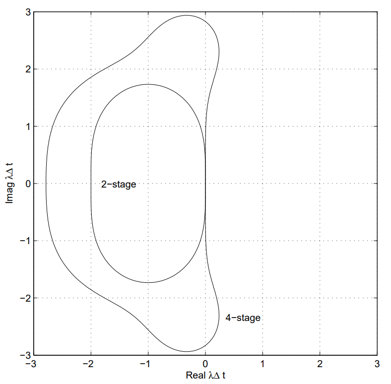
For reference, the stability regions of the 2nd and 4th order Runge-Kutta methods that we discussed are as follows:

Interpretation of the Linear Stability Condition

To interpret the linear stability condition, recall that the linearization of a system interprets the dynamics as locally being due to the Jacobian of the system. Thus

\[u' = f(u,p,t)\]

is locally equivalent to

\[u' = \frac{df}{du}u\]

You can understand the local behavior through diagonalizing this matrix. Therefore, the scalar for the linear stability analysis is performing an analysis on the eigenvalues of the Jacobian. The method will be stable if the largest eigenvalues of df/du are all within the stability limit. This means that stability effects are different throughout the solution of a nonlinear equation and are generally understood locally (though different more comprehensive stability conditions exist!).

Implicit Methods

If instead of the Euler method we defined $f$ to be evaluated at the future point, we would receive a method like:

\[u_{n+1} = u_n + \Delta t f(u_{n+1},p,t+\Delta t)\]

in which case, for the stability calculation we would have that

\[u_{n+1} = u_n + \Delta t \alpha u_n\]

or

\[(1-z) u_{n+1} = u_n\]

which means that

\[u_{n+1} = \frac{1}{1-z} u_n\]

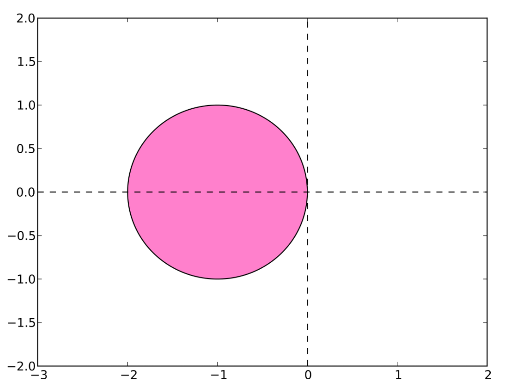
which is stable for all $Re(z) < 0$ a property which is known as A-stability. It is also stable as $z \rightarrow \infty$, a property known as L-stability. This means that for equations with very ill-conditioned Jacobians, this method is still able to be use reasonably large stepsizes and can thus be efficient.

Understanding Stiffness and the Relationship to DAEs

Stiffness and Timescale Separation

From this we see that there is a maximal stepsize whenever the eigenvalues of the Jacobian are sufficiently large. It turns out that's not an issue if the phenomena we see are fast, since then the total integration time tends to be small. However, if we have some equations with both fast modes and slow modes, like the Robertson equation (shown below), then it is very difficult because in order to resolve the slow dynamics over a long timespan, one needs to ensure that the fast dynamics do not diverge. This is a property known as stiffness. Stiffness can thus be approximated in some sense by the condition number of the Jacobian. The condition number of a matrix is its maximal eigenvalue divided by its minimal eigenvalue and gives a rough measure of the local timescale separations. If this value is large and one wants to resolve the slow dynamics, then explicit integrators, like the explicit Runge-Kutta methods described before, have issues with stability. In this case implicit integrators (or other forms of stabilized stepping) are required in order to efficiently reach the end time step.

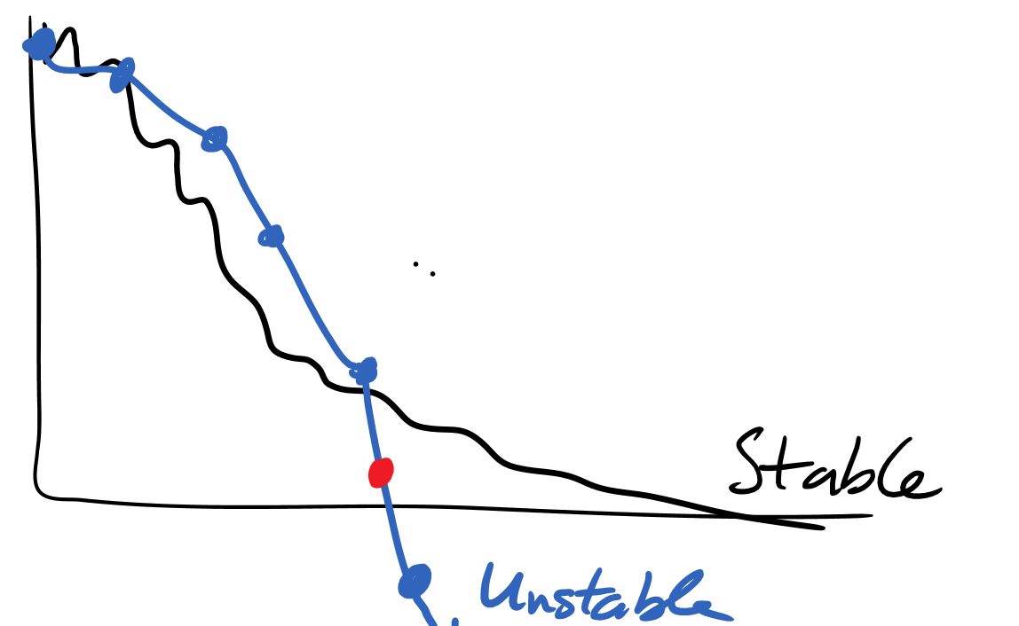
In this illustrative plot, the grey is "the true solution". The representative solution has a fast process and a slow process, the slow precess is an r-shaped curve. The fast process is a quasi-steady state process, i.e. it very quickly brings any purturbation from the r-shaped curve back to the main curve (and example of this is the $y_2$ term in the Robertson equation below). The black line up top is a numerical solution with an explicit method on such an equation. It's show how for a "reasonable" sized $h$ that the large derivatives of the fast process back to the stable manifold cause explicit methods to overshoot the manifold, thus requiring the $h$ to be small enough to "not overshoot too much", with this overshooting resulting in a jagged behavior.

This overshooting is exactly the behavior that causes a step size limitation, thus forcing $h$ to be sufficiently small when there is such time-scale separation, and thus simulations of the long-scale phonomena require time steps on the scale of the short-scale phonomena. If those two time-scales are orders of magnitude different, then accurately handling this type of equations thus requires orders of magnitude more time steps, leading to the inefficiency of explicit methods.

Implicit methods on the other hand effectively smooth out the behavior of the derivative in the future to be able to account for how the process had gotten there. For example, the red dotted line shows the linear extrapolation of the derivative from $t_n$ to $t_{n+1}$. But at the proposed $y_{n+1}$ of the Euler method, the derivative would be negative, and thus implicit Euler we detect a mismatch between the proposed value of $y_{n+1}$ and the required derivative to get to $y_{n+1}$. The solution of the implicit equation is thus an iterative process to remove this mismatch, which effectively smooths out the derivative issues and forces the solution onto the slow manifold.

Stiffness in Biochemistry: Robertson Equations

Biochemical equations commonly display large separation of timescales which lead to a stiffness phenomena that will be investigated later. The classic "hard" equations for ODE integration thus tend to come from biology (not physics!) due to this property. One of the standard models is the Robertson model, which can be described as:

using DifferentialEquations, Plots
function rober(du,u,p,t)
  y₁,y₂,y₃ = u
  k₁,k₂,k₃ = p
  du[1] = -k₁*y₁+k₃*y₂*y₃
  du[2] =  k₁*y₁-k₂*y₂^2-k₃*y₂*y₃
  du[3] =  k₂*y₂^2
end
prob = ODEProblem(rober,[1.0,0.0,0.0],(0.0,1e5),(0.04,3e7,1e4))
sol = solve(prob,Rosenbrock23())
plot(sol)

plot(sol, xscale=:log10, tspan=(1e-6, 1e5), layout=(3,1))

Stiffness in Chemical Physics: Pollution Models

Chemical reactions in physical models are also described as differential equation systems. The following is a classic model of dynamics between different species of pollutants:

k1=.35e0
k2=.266e2
k3=.123e5
k4=.86e-3
k5=.82e-3
k6=.15e5
k7=.13e-3
k8=.24e5
k9=.165e5
k10=.9e4
k11=.22e-1
k12=.12e5
k13=.188e1
k14=.163e5
k15=.48e7
k16=.35e-3
k17=.175e-1
k18=.1e9
k19=.444e12
k20=.124e4
k21=.21e1
k22=.578e1
k23=.474e-1
k24=.178e4
k25=.312e1
p = (k1,k2,k3,k4,k5,k6,k7,k8,k9,k10,k11,k12,k13,k14,k15,k16,k17,k18,k19,k20,k21,k22,k23,k24,k25)
function f(dy,y,p,t)
 k1,k2,k3,k4,k5,k6,k7,k8,k9,k10,k11,k12,k13,k14,k15,k16,k17,k18,k19,k20,k21,k22,k23,k24,k25 = p
 r1  = k1 *y[1]
 r2  = k2 *y[2]*y[4]
 r3  = k3 *y[5]*y[2]
 r4  = k4 *y[7]
 r5  = k5 *y[7]
 r6  = k6 *y[7]*y[6]
 r7  = k7 *y[9]
 r8  = k8 *y[9]*y[6]
 r9  = k9 *y[11]*y[2]
 r10 = k10*y[11]*y[1]
 r11 = k11*y[13]
 r12 = k12*y[10]*y[2]
 r13 = k13*y[14]
 r14 = k14*y[1]*y[6]
 r15 = k15*y[3]
 r16 = k16*y[4]
 r17 = k17*y[4]
 r18 = k18*y[16]
 r19 = k19*y[16]
 r20 = k20*y[17]*y[6]
 r21 = k21*y[19]
 r22 = k22*y[19]
 r23 = k23*y[1]*y[4]
 r24 = k24*y[19]*y[1]
 r25 = k25*y[20]

 dy[1]  = -r1-r10-r14-r23-r24+
          r2+r3+r9+r11+r12+r22+r25
 dy[2]  = -r2-r3-r9-r12+r1+r21
 dy[3]  = -r15+r1+r17+r19+r22
 dy[4]  = -r2-r16-r17-r23+r15
 dy[5]  = -r3+r4+r4+r6+r7+r13+r20
 dy[6]  = -r6-r8-r14-r20+r3+r18+r18
 dy[7]  = -r4-r5-r6+r13
 dy[8]  = r4+r5+r6+r7
 dy[9]  = -r7-r8
 dy[10] = -r12+r7+r9
 dy[11] = -r9-r10+r8+r11
 dy[12] = r9
 dy[13] = -r11+r10
 dy[14] = -r13+r12
 dy[15] = r14
 dy[16] = -r18-r19+r16
 dy[17] = -r20
 dy[18] = r20
 dy[19] = -r21-r22-r24+r23+r25
 dy[20] = -r25+r24
end

f (generic function with 1 method)

u0 = zeros(20)
u0[2]  = 0.2
u0[4]  = 0.04
u0[7]  = 0.1
u0[8]  = 0.3
u0[9]  = 0.01
u0[17] = 0.007
prob = ODEProblem(f,u0,(0.0,60.0),p)
sol = solve(prob,Rodas5P())

retcode: Success
Interpolation: specialized 4rd order "free" stiffness-aware interpolation
t: 30-element Vector{Float64}:
  0.0
  0.0013845590497824308
  0.003248154820240184
  0.007822056050945408
  0.015636473638329054
  0.02695092961815919
  0.04478922697244149
  0.07253076423642746
  0.10600967847261421
  0.1550976378543455
  ⋮
  4.01833703454483
  6.080137864970215
  9.234700036095719
 13.866865088960092
 20.139834368542314
 28.57562540061639
 39.68150334392996
 54.143352797090735
 60.0
u: 30-element Vector{Vector{Float64}}:
 [0.0, 0.2, 0.0, 0.04, 0.0, 0.0, 0.1, 0.3, 0.01, 0.0, 0.0, 0.0, 0.0, 0.0, 0.0, 0.0, 0.007, 0.0, 0.0, 0.0]
 [0.00029350835599164127, 0.1997064910246462, 1.6933646659442256e-10, 0.03970673366396415, 1.142760852742035e-7, 1.0934662220568216e-7, 0.09999966675482728, 0.30000033504926327, 0.009999982097053323, 5.608275186090612e-9, 6.0437672559379115e-9, 1.0053303376429798e-8, 5.95030281349918e-12, 6.2407891504614965e-9, 2.3086790312357436e-10, 3.129330571410992e-17, 0.0069999994176068725, 5.823931280628732e-10, 3.824053725159255e-10, 6.931199753689511e-14]
 [0.0006848307393263268, 0.19931516395991847, 1.9614145270676562e-10, 0.03931628333733633, 2.0845795047203617e-7, 2.527988735396753e-7, 0.0999988378095226, 0.3000011665225655, 0.009999897119251894, 2.064534412752599e-8, 1.687305270628739e-8, 8.167731332135961e-8, 1.0779517325590447e-10, 6.514505502657275e-8, 3.1173973981561673e-9, 3.0985586958414323e-17, 0.006999996431845442, 3.5681545580507224e-9, 2.07143920473889e-9, 2.061752236742482e-12]
 [0.001626673842789779, 0.19837327663367996, 2.61341517186769e-10, 0.03837837135119767, 3.499140256138006e-7, 4.640939891340906e-7, 0.0999955180524943, 0.3000044941971509, 0.009999482640907172, 4.469079614092972e-8, 3.316652483724116e-8, 4.7262219296034596e-7, 1.4018895300664164e-9, 4.360187226554445e-7, 3.646907321606834e-8, 3.0246408405940866e-17, 0.0069999816561534, 1.8343846600048992e-8, 1.1520193471079965e-8, 6.618705754098527e-11]
 [0.0031739598368824284, 0.19682578480247068, 3.6848274612582107e-10, 0.036840444265251716, 4.308058894245777e-7, 5.770922655811164e-7, 0.09998792362054168, 0.3000121120820022, 0.009998465300944014, 5.828043759889608e-8, 4.216064737085081e-8, 1.4641454855949606e-6, 8.066719707030999e-9, 1.4108149108097597e-6, 2.0286586083895822e-7, 2.9034351481624044e-17, 0.006999945226182863, 5.477381713749204e-8, 4.248810508564416e-8, 9.699806494900167e-10]
 [0.00527985593453901, 0.1947193383531825, 5.143418506781766e-10, 0.0347488996031483, 4.3093601952954417e-7, 5.646226467930153e-7, 0.09997626842071211, 0.3000238282736904, 0.009996882519830105, 5.7928612826073366e-8, 4.16241161501318e-8, 3.0144643408683243e-6, 2.636014341246327e-8, 2.9299044645063637e-6, 6.539227913561269e-7, 2.738598257429025e-17, 0.006999888501592138, 1.1149840786279859e-7, 1.1048653161793254e-7, 7.471406060555517e-9]
 [0.008303332733066323, 0.19169456572579305, 7.237922059569431e-10, 0.03174600330420883, 3.979588459244406e-7, 4.999453551109529e-7, 0.09995919302644539, 0.30004106184979734, 0.0099945852514614, 5.172437268072286e-8, 3.7108987770252254e-8, 5.250222785609308e-6, 6.920535643683605e-8, 5.060044987751721e-6, 1.7029563673086802e-6, 2.501936761224585e-17, 0.006999806222084552, 1.9377791544810596e-7, 2.393708350642762e-7, 4.500429091005969e-8]
 [0.012381216304727582, 0.18761393275867358, 1.0062796343688567e-9, 0.027695563423620763, 3.63737037857065e-7, 4.315804004432719e-7, 0.09993562728428845, 0.300065000639491, 0.009991470600090027, 4.5086072920571806e-8, 3.231183314858193e-8, 8.244514171660123e-6, 1.5832377775460823e-7, 7.760004574102389e-6, 3.869130998427598e-6, 2.1827172254836282e-17, 0.006999694805205503, 3.0519479449815307e-7, 4.0869403799383373e-7, 2.0739389231717105e-7]
 [0.016470145074437254, 0.18352084921518833, 1.289448860116361e-9, 0.023635066176169506, 3.408363434174163e-7, 3.823025203747643e-7, 0.09991026515233849, 0.3000909794121657, 0.009988177497437328, 4.0347996010672295e-8, 2.8879229651845425e-8, 1.136510631334099e-5, 2.9078873481039145e-7, 1.0355650382795339e-5, 7.062384503143422e-6, 1.8627050578125932e-17, 0.006999577163514119, 4.228364858828224e-7, 5.064584290101607e-7, 5.730393537301469e-7]
 [0.021191772350648914, 0.17879211720086433, 1.6163236315104805e-9, 0.0189497541387097, 3.233310106833691e-7, 3.4022871811801787e-7, 0.09987670742311801, 0.3001256997501773, 0.009983888194513471, 3.634759463668129e-8, 2.597408219749891e-8, 1.5366225206057014e-5, 5.18152958037098e-7, 1.332561079652248e-5, 1.2493270736175514e-5, 1.493450562624091e-17, 0.006999424135598123, 5.758644018788993e-7, 5.168278330665833e-7, 1.291098479734196e-6]
 ⋮
 [0.03909671115400585, 0.16021388214020088, 2.863393797290316e-9, 0.0031978042762335662, 3.0843925599405756e-7, 2.588368231701203e-7, 0.09791348199751557, 0.30230016229129175, 0.009735232023433897, 2.868786924051746e-8, 2.0384970968272198e-8, 0.0002330184586693148, 2.6577021690955245e-5, 2.9649704462246316e-5, 0.0006371402432266941, 2.5202240411657423e-18, 0.006990490567780576, 9.509432219422943e-6, 5.814540574029035e-7, 1.2553993409201942e-5]
 [0.04007594328989523, 0.15887797935273862, 2.9352999831810086e-9, 0.0033061459028971988, 3.0068637733707693e-7, 2.504304876371835e-7, 0.09692151124673885, 0.30340723091376903, 0.009610779514983223, 2.7692637623148513e-8, 1.9663322731706254e-8, 0.0003416805573576498, 3.977558338946253e-5, 2.840006610578639e-5, 0.0009758574296736734, 2.6056092456968673e-18, 0.006985941923970138, 1.405807602985967e-5, 6.65286868027656e-7, 1.4889528717591963e-5]
 [0.0414930713952667, 0.1569236564001045, 3.039341535694452e-9, 0.0034666133154929975, 2.898631533374969e-7, 2.387643153577775e-7, 0.09546210819138151, 0.3050336473820511, 0.009430661992494614, 2.6329882649136633e-8, 1.8675357206607864e-8, 0.0004991324605025568, 5.853821267927339e-5, 2.6647875119831033e-5, 0.0014885730747294943, 2.7320753443425123e-18, 0.006979264491790816, 2.0735508209182298e-5, 7.587613195129447e-7, 1.77010779503414e-5]
 [0.043416636083269844, 0.15422706616750667, 3.180570155809784e-9, 0.0036919031761507366, 2.7613029280705503e-7, 2.2401971337643903e-7, 0.09343238864267965, 0.3072912798514192, 0.009185840124906988, 2.4636441831344505e-8, 1.744801635899646e-8, 0.0007136662086042755, 8.322339134897651e-5, 2.4478732310215853e-5, 0.00222970741931009, 2.9096287134715613e-18, 0.006970003005636785, 2.999699436321478e-5, 8.674683665258634e-7, 2.1249735099046842e-5]
 [0.04576994195589239, 0.15085317855916136, 3.3533971788025496e-9, 0.003980365145865279, 2.6061559981020415e-7, 2.074588530091386e-7, 0.09086737982791197, 0.31013781522691053, 0.008885404597732977, 2.277372099981477e-8, 1.6098530016404735e-8, 0.000978087639936781, 0.0001118726206466993, 2.2107897700089242e-5, 0.003212277486458904, 3.1369687031137414e-18, 0.006958331427300152, 4.1668572699848246e-5, 9.995840133870664e-7, 2.586489691375637e-5]
 [0.048565491423233624, 0.14672814420651925, 3.5587955651609294e-9, 0.0043436377290348, 2.436885249154007e-7, 1.8954702477757186e-7, 0.08769384121091091, 0.3136509304063337, 0.008526637098039115, 2.0805075712340766e-8, 1.4673027610821725e-8, 0.0012960907515314885, 0.00014309518242210212, 1.9622919170204742e-5, 0.004497745363779089, 3.4232677441165217e-18, 0.006943923280400517, 5.607671959948275e-5, 1.1700945109085837e-6, 3.21768647676605e-5]
 [0.05174083432863735, 0.1418706120130952, 3.792244805244997e-9, 0.00478756515261096, 2.260144308047927e-7, 1.7108314017697025e-7, 0.08390461967970261, 0.31783475059500227, 0.00811565776886708, 1.882072909515642e-8, 1.3237032070355706e-8, 0.0016641981445851158, 0.00017396213714284656, 1.7146473896493043e-5, 0.006131731292169565, 3.773131734775514e-18, 0.006926739428155184, 7.326057184481697e-5, 1.3884790514943577e-6, 4.073587495191291e-5]
 [0.055221414196813166, 0.13630373356524159, 4.0483477151717606e-9, 0.005319807138831808, 2.080450144241726e-7, 1.5265565180019845e-7, 0.07949158728346996, 0.32269460942172196, 0.00765898912844823, 1.6873902325216683e-8, 1.1829162157896872e-8, 0.002079000018354831, 0.00020101384715833485, 1.475679301301915e-5, 0.008167859927842944, 4.192597384803209e-18, 0.006906714474258816, 9.328552574118534e-5, 1.6636577728168648e-6, 5.2157402585685636e-5]
 [0.056462553323845074, 0.13424841358635414, 4.139734221239658e-9, 0.005523140190492613, 2.0189768077835197e-7, 1.4645415660794528e-7, 0.07784249229110898, 0.3245075344177776, 0.007494013207038758, 1.622292918349514e-8, 1.1358636563258352e-8, 0.002230506106738904, 0.00020871632118130894, 1.3969187731602392e-5, 0.008964885874226987, 4.352846355938725e-18, 0.006899219697884304, 0.00010078030211569819, 1.7721447337603926e-6, 5.682937482947947e-5]

plot(sol)

plot(sol, xscale=:log10, tspan=(1e-6, 60), layout=(3,1))

Van Der Pol Equations: Singular Perturbation Problems and DAEs

Next up is the Van Der Pol Equations which is a canonical example of a singular perturbation problem:

function van(du,u,p,t)
    y,x = u
    μ = p
    du[1] = μ*((1-x^2)*y - x)
    du[2] = 1*y
end

prob = ODEProblem(van,[1.0;1.0],(0.0,6.3),1e6)
sol = solve(prob, Rodas5P())
plot(sol)

or zooming in:

plot(sol, ylim=[-4;4])

A singular perturbation problem is an ODE given by the form:

\[x' = f(x,y,t)\\ \epsilon y' = g(x,y,t)\]

where $\epsilon$ is sufficiently small. Notice that the Van Der Pol equations,

\[x' = y\\ y' = \mu ((1-x^2)y -x)\]

can be rewritten as:

\[x' = y\\ \epsilon y' = (1-x^2)y -x\]

by making $\epsilon = \frac{1}{\mu}$. Thus when $\mu$ is big, $\epsilon$ is small. In this form it's clear that $\epsilon$ is the time-scale difference between the changes in $x$ and the changes in $y$. When this difference is large, i.e. $\mu$ is big, then our previous discussion suggests that this should change the stiffness. Let's see this in practice:

# small mu
prob = ODEProblem(van,[1.0;1.0],(0.0,6.3),500)
# explicit RK solution
sol = solve(prob,Tsit5())
plot(sol, ylim=[-4;4])

# big mu
prob = ODEProblem(van,[1.0;1.0],(0.0,6.3),1e6)
# explicit RK solution
sol = solve(prob,Tsit5())

retcode: MaxIters
Interpolation: specialized 4th order "free" interpolation
t: 999967-element Vector{Float64}:
 0.0
 1.4142135623723879e-6
 1.5556349186096265e-5
 5.064808332629735e-5
 9.141714346641453e-5
 0.00013159621249585464
 0.0001643364000193749
 0.0001814117752651743
 0.00019048244999619597
 0.00019562813286395545
 ⋮
 1.8454390443485207
 1.8454405286737303
 1.8454420130016336
 1.8454434973322302
 1.8454449816654221
 1.8454464660012093
 1.8454479503395917
 1.845449434680766
 1.8454509190246338
u: 999967-element Vector{Vector{Float64}}:
 [1.0, 1.0]
 [-0.4142142625400887, 1.0000004142130319]
 [-14.566967050424426, 0.9998945259848284]
 [-51.181954238945295, 0.9987529979984154]
 [-109.7644012955115, 0.9955835526886252]
 [-253.72726534691068, 0.9888631462607406]
 [-834.7745679124318, 0.9739545463817227]
 [-2872.4860041203997, 0.947638008236739]
 [-10069.848884501966, 0.8988637843697357]
 [-38569.75311229706, 0.7971021527741678]
 ⋮
 [0.7758666698780496, -1.8337363813628822]
 [0.7758675699617644, -1.8337352292955171]
 [0.7758684700026367, -1.833734077224725]
 [0.7758693700006768, -1.833732925150506]
 [0.7758702700765642, -1.8337317730729359]
 [0.7758711702303155, -1.833730620992015]
 [0.7758720704619425, -1.8337294689077432]
 [0.7758729705301266, -1.833728316819968]
 [0.7758738705555462, -1.8337271647287656]

We can see directly that the time scale separation forces the explicit Runge-Kutta method to exit with MaxIters, i.e. it hit its maximum iterations. The reason why it hit maximum iterations is because the time scale separation increased, and therefore the dt limit for stability decreased, and therefore it started requiring too many steps (default 1e5) in order to solve the equation.

Notably, this shows that stiffness is a parameter-dependent phonomena

If you change the parameter values, you can change whether an equation is stiff or non-stiff.

However... what happens in the limit as $\mu \rightarrow \infty$? In some sense, this is "the limit as stiffness goes to infinity". In that limit, $\epsilon \rightarrow 0$, and therefore we arrive at the equation:

\[x' = y\\ 0 = (1-x^2)y - x\]

This equation is a Differential-Algebraic Equation (DAE), where $x' = y$ is a differential equation and $0 = (1-x^2)y -x$ is a nonlinear algebraic equation. In this limit, the fast behavior is so fast that it's instant. Thinking back to our picture of stiffness, it means any perturbation from the slow manifold would instantly fall back onto the slow manifold. For these types of problem then, it's clear that handling the equation implicitly is potentially required for two reasons. For one, it's infinitely stiff, and the "more stiff" an equation is, the more one requires using implicit methods

Representations of DAEs as Mass Matrix ODEs

Take Van Der Pol's Equation

\[x' = y\\ 0 = (1-x^2)y - x\]

In order to more succinctly represent this to an ODE solver, notice that if we take the mass matrix [1 0;0 0], then the form:

\[Mu' = f(u,t)\]

is a representation of the Van Der Pol equation. Notably, the "standard" ODE from before is of the same form, simply with $M = I$. If the mass matrix $M$ is non-singular, then the equation is a mass matrix ODE which does not represent a DAE. However, if $M$ is singular, then the equation is implicitly specifying an algebraic equation, like as in the Van Der Pol equation, and its in this case that a mass matrix ODE is representing a DAE.

The Three Canonical Representations of DAEs

This shows the three canonical ways that DAEs can be represented. The first is the semi-explicit ODE in the split function form:

\[x' = f(x,y,t)\\ 0 = g(x,y,t)\]

where $x$ are the differential variables (generally a vector) and $y$ is a vector of algebraic variables. The second form is the mass matrix ODE form:

\[Mu' = f(u,t)\]

where the mass matrix $M$ is singular. In this form, the algebraic equations can be sometimes easily understood via a constant zero row in the mass matrix $M$, with the differential variables being the values for which the derivative appears in the equation and the other variables being the algebraic variables. Note that this description is purposefully vague as we will see that not all equations can be cleanly separated like this in the more general forms.

Finally, the most general form is simply the implicit ODE form:

\[0 = f(u',u,t)\]

This form is slightly more general since one can consider the mass matrix form as requiring that $f(u',u,t)$ has a linear partial derivative with respect to the $u'$ term, with $-M$ being that derivative. Thus it allows for example $u_1'^2$.

Though note that the mass matrix and the implicit ODE definitions are not a substantial difference as via a variable definition $u_i = u_1^3$ and other tricks you can rewrite a term with nonlinear derivatives into one with linear derivative relationships, and thus arrive at a mass matrix form (with a larger set of equations). The semi-explicit ODE however is distinctly a subset of the possible DAEs, which will be explored in the symbolic sections in more detail.

The Steps of an Implicit Solver

Newton's Method and Jacobians

Recall that the implicit Euler method is the following:

\[u_{n+1} = u_n + \Delta t f(u_{n+1},p,t + \Delta t)\]

If we wanted to use this method, we would need to find out how to get the value $u_{n+1}$ when only knowing the value $u_n$. To do so, we can move everything to one side:

\[u_{n+1} - \Delta t f(u_{n+1},p,t + \Delta t) - u_n = 0\]

and now we have a problem

\[g(u_{n+1}) = 0\]

This is the classic rootfinding problem $g(x)=0$, find $x$. The way that we solve the rootfinding problem is, once again, by replacing this problem about a continuous function $g$ with a discrete dynamical system whose steady state is the solution to the $g(x)=0$. There are many methods for this, but some choices of the rootfinding method effect the stability of the ODE solver itself since we need to make sure that the steady state solution is a stable steady state of the iteration process, otherwise the rootfinding method will diverge (will be explored in the homework).

Thus for example, fixed point iteration is not appropriate for stiff differential equations. Methods which are used in the stiff case are either Anderson Acceleration or Newton's method. Newton's is by far the most common (and generally performs the best), so we can go down this route.

Let's use the syntax $g(x)=0$. Here we need some starting value $x_0$ as our first guess for $u_{n+1}$. The easiest guess is $u_{n}$, though additional information about the equation can be used to compute a better starting value (known as a step predictor). Once we have a starting value, we run the iteration:

\[x_{k+1} = x_k - J(x_k)^{-1}g(x_k)\]

where $J(x_k)$ is the Jacobian of $g$ at the point $x_k$. However, the mathematical formulation is never the syntax that you should use for the actual application! Instead, numerically this is two stages:

• Solve $Ja=g(x_k)$ for $a$
• Update $x_{k+1} = x_k - a$

By doing this, we can turn the matrix inversion into a problem of a linear solve and then an update. The reason this is done is manyfold, but one major reason is because the inverse of a sparse matrix can be dense, and this Jacobian is in many cases (PDEs) a large and dense matrix.

Now let's break this down step by step.

Some Quick Notes

The Jacobian of $g$ can also be written as $J = I - \gamma \frac{df}{du}$ for the ODE $u' = f(u,p,t)$, where $\gamma = \Delta t$ for the implicit Euler method. This general form holds for all other (SDIRK) implicit methods, changing the value of $\gamma$. Additionally, the class of Rosenbrock methods solves a linear system with exactly the same $J$, meaning that essentially all implicit and semi-implicit ODE solvers have to do the same Newton iteration process on the same structure. This is the portion of the code that is generally the bottleneck.

Additionally, if one is solving a mass matrix ODE: $Mu' = f(u,p,t)$, exactly the same treatment can be had with $J = M - \gamma \frac{df}{du}$. This works even if $M$ is singular, a case known as a differential-algebraic equation or a DAE. A DAE for example can be an ODE with constraint equations, and these structures can be represented as an ODE where these constraints lead to a singularity in the mass matrix (a row of all zeros is a term that is only the right hand side equals zero!).

Generation of the Jacobian

Dense Finite Differences and Forward-Mode AD

Recall that the Jacobian is the matrix of $\frac{df_i}{dx_j}$ for $f$ a vector-valued function. The simplest way to generate the Jacobian is through finite differences. For each $h_j = h e_j$ for $e_j$ the basis vector of the $j$th axis and some sufficiently small $h$, then we can compute column $j$ of the Jacobian by:

\[\frac{f(x+h_j)-f(x)}{h}\]

Thus $m+1$ applications of $f$ are required to compute the full Jacobian.

This can be improved by using forward-mode automatic differentiation. Recall that we can formulate a multidimensional duel number of the form

\[d = x + v_1 \epsilon_1 + \ldots + v_m \epsilon_m\]

We can then seed the vectors $v_j = h_j$ so that the differentiation directions are along the basis vectors, and then the output dual is the result:

\[f(d) = f(x) + J_1 \epsilon_1 + \ldots + J_m \epsilon_m\]

where $J_j$ is the $j$th column of the Jacobian. And thus with one calculation of the primal (f(x)) we have calculated the entire Jacobian.

Sparse Differentiation and Matrix Coloring

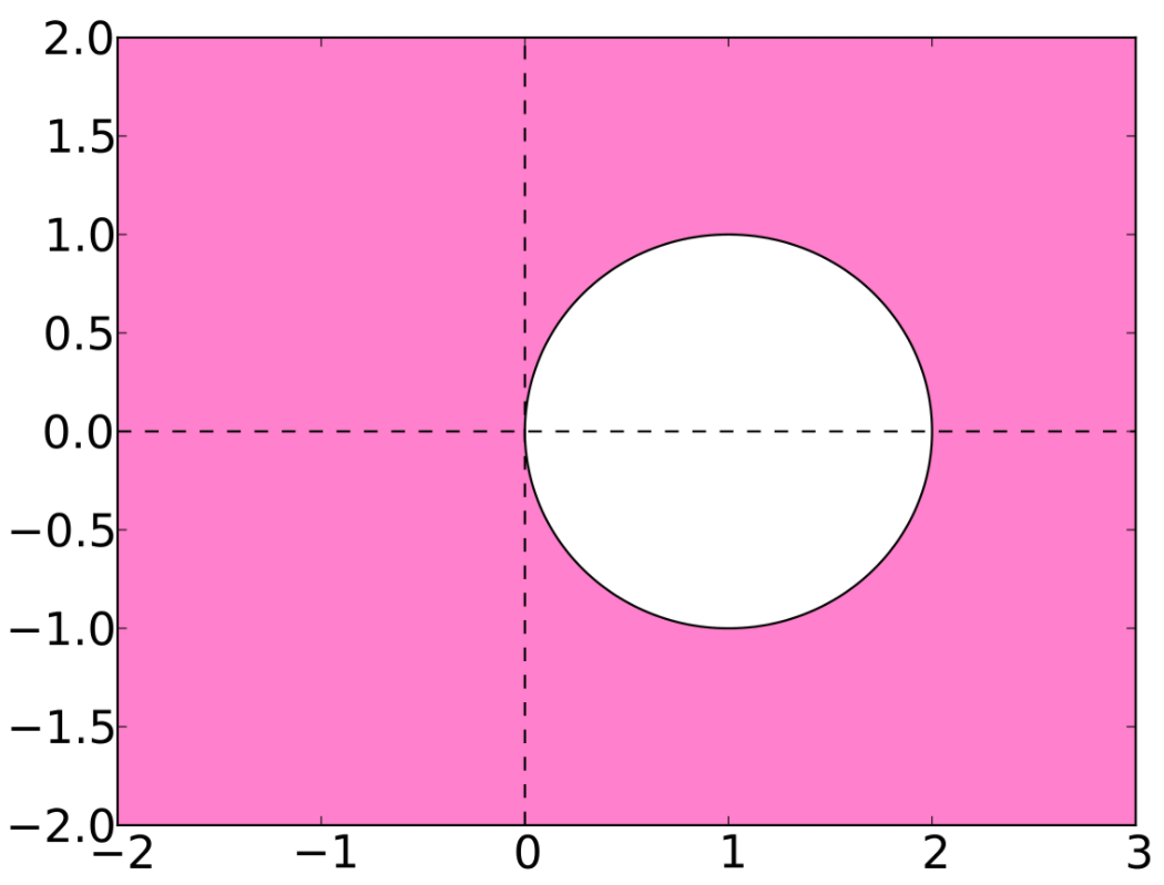
However, when the Jacobian is sparse we can compute it much faster. We can understand this by looking at the following system:

\[f(x)=\left[\begin{array}{c} x_{1}+x_{3}\\ x_{2}x_{3}\\ x_{1} \end{array}\right]\]

Notice that in 3 differencing steps we can calculate:

\[f(x+\epsilon e_{1})=\left[\begin{array}{c} x_{1}+x_{3}+\epsilon\\ x_{2}x_{3}\\ x_{1}+\epsilon \end{array}\right]\]

\[f(x+\epsilon e_{2})=\left[\begin{array}{c} x_{1}+x_{3}\\ x_{2}x_{3}+\epsilon x_{3}\\ x_{1} \end{array}\right]\]

\[f(x+\epsilon e_{3})=\left[\begin{array}{c} x_{1}+x_{3}+\epsilon\\ x_{2}x_{3}+\epsilon x_{2}\\ x_{1} \end{array}\right]\]

and thus:

\[\frac{f(x+\epsilon e_{1})-f(x)}{\epsilon}=\left[\begin{array}{c} 1\\ 0\\ 1 \end{array}\right]\]

\[\frac{f(x+\epsilon e_{2})-f(x)}{\epsilon}=\left[\begin{array}{c} 0\\ x_{3}\\ 0 \end{array}\right]\]

\[\frac{f(x+\epsilon e_{3})-f(x)}{\epsilon}=\left[\begin{array}{c} 1\\ x_{2}\\ 0 \end{array}\right]\]

But notice that the calculation of $e_1$ and $e_2$ do not interact. If we had done:

\[\frac{f(x+\epsilon e_{1}+\epsilon e_{2})-f(x)}{\epsilon}=\left[\begin{array}{c} 1\\ x_{3}\\ 1 \end{array}\right]\]

we would still get the correct value for every row because the $\epsilon$ terms do not collide (a situation known as perturbation confusion). If we knew the sparsity pattern of the Jacobian included a 0 at (2,1), (1,2), and (3,2), then we would know that the vectors would have to be $[1 0 1]$ and $[0 x_3 0]$, meaning that columns 1 and 2 can be computed simultaneously and decompressed. This is the key to sparse differentiation.

With forward-mode automatic differentiation, recall that we calculate multiple dimensions simultaneously by using a multidimensional dual number seeded by the vectors of the differentiation directions, that is:

\[d = x + v_1 \epsilon_1 + \ldots + v_m \epsilon_m\]

Instead of using the primitive differentiation directions $e_j$, we can instead replace this with the mixed values. For example, the Jacobian of the example function can be computed in one function call to $f$ with the dual number input:

\[d = x + (e_1 + e_2) \epsilon_1 + e_3 \epsilon_2\]

and performing the decompression via the sparsity pattern. Thus the sparsity pattern gives a direct way to optimize the construction of the Jacobian.

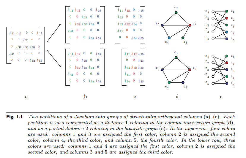
This idea of independent directions can be formalized as a matrix coloring. Take $S_{ij}$ the sparsity pattern of some Jacobian matrix $J_{ij}$. Define a graph on the nodes 1 through m where there is an edge between $i$ and $j$ if there is a row where $i$ and $j$ are non-zero. This graph is the column connectivity graph of the Jacobian. What we wish to do is find the smallest set of differentiation directions such that differentiating in the direction of $e_i$ does not collide with differentiation in the direction of $e_j$. The connectivity graph is setup so that way this cannot be done if the two nodes are adjacent. If we let the subset of nodes differentiated together be a color, the question is, what is the smallest number of colors s.t. no adjacent nodes are the same color. This is the classic distance-1 coloring problem from graph theory. It is well-known that the problem of finding the chromatic number, the minimal number of colors for a graph, is generally NP-complete. However, there are heuristic methods for performing a distance-1 coloring quite quickly. For example, a greedy algorithm is as follows:

• Pick a node at random to be color 1.
• Make all nodes adjacent to that be the lowest color that they can be (in this step that will be 2).
• Now look at all nodes adjacent to that. Make all nodes be the lowest color that they can be (either 1 or 3).
• Repeat by looking at the next set of adjacent nodes and color as conservatively as possible.

This can be visualized as follows:

The result will color the entire connected component. While not giving an optimal result, it will still give a result that is a sufficient reduction in the number of differentiation directions (without solving an NP-complete problem) and thus can lead to a large computational saving.

At the end, let $c_i$ be the vector of 1's and 0's, where it's 1 for every node that is color $i$ and 0 otherwise. Sparse automatic differentiation of the Jacobian is then computed with:

\[d = x + c_1 \epsilon_1 + \ldots + c_k \epsilon_k\]

that is, the full Jacobian is computed with one dual number which consists of the primal calculation along with $k$ dual dimensions, where $k$ is the computed chromatic number of the connectivity graph on the Jacobian. Once this calculation is complete, the colored columns can be decompressed into the full Jacobian using the sparsity information, generating the original quantity that we wanted to compute.

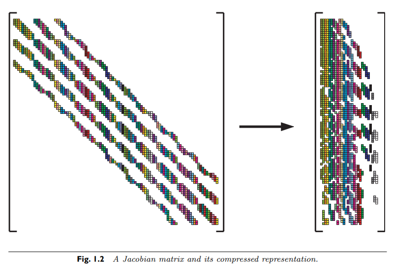
For more information on the graph coloring aspects, find the paper titled "What Color Is Your Jacobian? Graph Coloring for Computing Derivatives" by Gebremedhin.

Note on Sparse Reverse-Mode AD

Reverse-mode automatic differentiation can be though of as a method for computing one row of a Jacobian per seed, as opposed to one column per seed given by forward-mode AD. Thus sparse reverse-mode automatic differentiation can be done by looking at the connectivity graph of the column and using the resulting color vectors to seed the reverse accumulation process.

Linear Solving

After the Jacobian has been computed, we need to solve a linear equation $Ja=b$. While mathematically you can solve this by computing the inverse $J^{-1}$, this is not a good way to perform the calculation because even if $J$ is sparse, then $J^{-1}$ is in general dense and thus may not fit into memory (remember, this is $N^2$ as many terms, where $N$ is the size of the ordinary differential equation that is being solved, so if it's a large equation it is very feasible and common that the ODE is representable but its full Jacobian is not able to fit into RAM). Note that some may say that this is done for numerical stability reasons: that is incorrect. In fact, under reasonable assumptions for how the inverse is computed, it will be as numerically stable as other techniques we will mention.

Thus instead of generating the inverse, we can instead perform a matrix factorization. A matrix factorization is a transformation of the matrix into a form that is more amenable to certain analyses. For our purposes, a general Jacobian within a Newton iteration can be transformed via the LU-factorization or (LU-decomposition), i.e.

\[J = LU\]

where $L$ is lower triangular and $U$ is upper triangular. If we write the linear equation in this form:

\[LUa = b\]

then we see that we can solve it by first solving $L(Ua) = b$. Since $L$ is lower triangular, this is done by the backsubstitution algorithm. That is, in a lower triangular form, we can solve for the first value since we have:

\[L_{11} a_1 = b_1\]

and thus by dividing we solve. For the next term, we have that

\[L_{21} a_1 + L_{22} a_2 = b_2\]

and thus we plug in the solution to $a_1$ and solve to get $a_2$. The lower triangular form allows this to continue. This occurs in 1+2+3+...+n operations, and is thus O(n^2). Next, we solve $Ua = b$, which once again is done by a backsubstitution algorithm but in the reverse direction. Together those two operations are O(n^2) and complete the inversion of $LU$.

So is this an O(n^2) algorithm for computing the solution of a linear system? No, because the computation of $LU$ itself is an O(n^3) calculation, and thus the true complexity of solving a linear system is still O(n^3). However, if we have already factorized $J$, then we can repeatedly use the same $LU$ factors to solve additional linear problems $Jv = u$ with different vectors. We can exploit this to accelerate the Newton method. Instead of doing the calculation:

\[x_{k+1} = x_k - J(x_k)^{-1}g(x_k)\]

we can instead do:

\[x_{k+1} = x_k - J(x_0)^{-1}g(x_k)\]

so that all of the Jacobians are the same. This means that a single O(n^3) factorization can be done, with multiple O(n^2) calculations using the same factorization. This is known as a Quasi-Newton method. While this makes the Newton method no longer quadratically convergent, it minimizes the large constant factor on the computational cost while retaining the same dynamical properties, i.e. the same steady state and thus the same overall solution. This makes sense for sufficiently large $n$, but requires sufficiently large $n$ because the loss of quadratic convergence means that it will take more steps to converge than before, and thus more $O(n^2)$ backsolves are required, meaning that the difference between factorizations and backsolves needs to be large enough in order to offset the cost of extra steps.

Note on Sparse Factorization

Note that LU-factorization, and other factorizations, have generalizations to sparse matrices where a symbolic factorization is utilized to compute a sparse storage of the values which then allow for a fast backsubstitution. More details are outside the scope of this course, but note that Julia and MATLAB will both use the library SuiteSparse in the background when lu is called on a sparse matrix.

Jacobian-Free Newton Krylov (JFNK)

An alternative method for solving the linear system is the Jacobian-Free Newton Krylov technique. This technique is broken into two pieces: the jvp calculation and the Krylov subspace iterative linear solver.

Jacobian-Vector Products as Directional Derivatives

We don't actually need to compute $J$ itself, since all that we actually need is the v = J*w. Is it possible to compute the Jacobian-Vector Product, or the jvp, without producing the Jacobian?

To see how this is done let's take a look at what is actually calculated. Written out in the standard basis, we have that:

\[w_i = \sum_{j}^{m} J_{ij} v_{j}\]

Now write out what $J$ means and we see that:

\[w_i = \sum_j^{m} \frac{df_i}{dx_j} v_j = \nabla f_i(x) \cdot v\]

that is, the $i$th component of $Jv$ is the directional derivative of $f_i$ in the direction $v$. This means that in general, the jvp $Jv$ is actually just the directional derivative in the direction of $v$, that is:

\[Jv = \nabla f \cdot v\]

and therefore it has another mathematical representation, that is:

\[Jv = \lim_{\epsilon \rightarrow 0} \frac{f(x+v \epsilon) - f(x)}{\epsilon}\]

From this alternative form it is clear that we can always compute a jvp with a single computation. Using finite differences, a simple approximation is the following:

\[Jv \approx \frac{f(x+v \epsilon) - f(x)}{\epsilon}\]

for non-zero $\epsilon$. Similarly, recall that in forward-mode automatic differentiation we can choose directions by seeding the dual part. Therefore, using the dual number with one partial component:

\[d = x + v \epsilon\]

we get that

\[f(d) = f(x) + Jv \epsilon\]

and thus a single application with a single partial gives the jvp.

Note on Reverse-Mode Automatic Differentiation

As noted earlier, reverse-mode automatic differentiation has its primitives compute rows of the Jacobian in the seeded direction. This means that the seeded reverse-mode call with the vector $v$ computes $v^T J$, that is the vector (transpose) Jacobian transpose, or vjp for short. When discussing parameter estimation and adjoints, this shorthand will be introduced as a way for using a traditionally machine learning tool to accelerate traditionally scientific computing tasks.

Krylov Subspace Methods For Solving Linear Systems

Basic Iterative Solver Methods

Now that we have direct access to quick calculations of $Jv$, how would we use this to solve the linear system $Jw = v$ quickly? This is done through iterative linear solvers. These methods replace the process of solving for a factorization with, you may have guessed it, a discrete dynamical system whose solution is $w$. To do this, what we want is some iterative process so that

\[Jw - b = 0\]

So now let's split $J = A - B$, then if we are iterating the vectors $w_k$ such that $w_k \rightarrow w$, then if we plug this into the previous (residual) equation we get

\[A w_{k+1} = Bw_k + b\]

since when we plug in $w$ we get zero (the sequence must be Cauchy so the difference $w_{k+1} - w_k \rightarrow 0$). Thus if we can split our matrix $J$ into a component $A$ which is easy to invert and a part $B$ that is just everything else, then we would have a bunch of easy linear systems to solve. There are many different choices that we can do. If we let $J = L + D + U$, where $L$ is the lower portion of $J$, $D$ is the diagonal, and $U$ is the upper portion, then the following are well-known methods:

• Richardson: $A = \omega I$ for some $\omega$
• Jacobi: $A = D$
• Damped Jacobi: $A = \omega D$
• Gauss-Seidel: $A = D-L$
• Successive Over Relaxation: $A = \omega D - L$
• Symmetric Successive Over Relaxation: $A = \frac{1}{\omega (2 - \omega)}(D-\omega L)D^{-1}(D-\omega U)$

These decompositions are chosen since a diagonal matrix is easy to invert (it's just the inversion of the scalars of the diagonal) and it's easy to solve an upper or lower triangular linear system (once again, it's backsubstitution).

Since these methods give a a linear dynamical system, we know that there is a unique steady state solution, which happens to be $Aw - Bw = Jw = b$. Thus we will converge to it as long as the steady state is stable. To see if it's stable, take the update equation

\[w_{k+1} = A^{-1}(Bw_k + b)\]

and check the eigenvalues of the system: if they are within the unit circle then you have stability. Notice that this can always occur by bringing the eigenvalues of $A^{-1}$ closer to zero, which can be done by multiplying $A$ by a significantly large value, hence the $\omega$ quantities. While that always works, this essentially amounts to decreasing the stepsize of the iterative process and thus requiring more steps, thus making it take more computations. Thus the game is to pick the largest stepsize ($\omega$) for which the steady state is stable. We will leave that as outside the topic of this course.

Krylov Subspace Methods

While the classical iterative solver methods give the background for understanding an alternative to direct inversion or factorization of a matrix, the problem with that approach is that it requires the ability to split the matrix $J$, which we would like to avoid computing. Instead, we would like to develop an iterative solver technique which instead just uses the solution to $Jv$. Indeed there are such methods, and these are the Krylov subspace methods. A Krylov subspace is the space spanned by:

\[\mathcal{K}_k = \text{span} \{v,Jv,J^2 v, \ldots, J^k v\}\]

There are a few nice properties about Krylov subspaces that can be exploited. For one, it is known that there is a finite maximum dimension of the Krylov subspace, that is there is a value $r$ such that $J^{r+1} v \in \mathcal{K}_r$, which means that the complete Krylov subspace can be computed in finitely many jvp, since $J^2 v$ is just the jvp where the vector is the jvp. Indeed, one can show that $J^i v$ is linearly independent for each $i$, and thus that maximal value is $m$, the dimension of the Jacobian. Therefore in $m$ jvps the solution is guaranteed to live in the Krylov subspace, giving a maximal computational cost and a proof of convergence if the vector in there is the "optimal in the space".

The most common method in the Krylov subspace family of methods is the GMRES method. Essentially, in step $i$ one computes $\mathcal{K}_i$, and finds the $x$ that is the closest to the Krylov subspace, i.e. finds the $x \in \mathcal{K}_i$ such that $\Vert Jx-v \Vert$ is minimized. At each step, it adds the new vector to the Krylov subspace after orthogonalizing it against the other vectors via Arnoldi iterations, leading to an orthogonal basis of $\mathcal{K}_i$ which makes it easy to express $x$.

While one has a guaranteed bound on the number of possible jvps in GMRES which is simply the number of ODEs (since that is what determines the size of the Jacobian and thus the total dimension of the problem), that bound is not necessarily a good one. For a large sparse matrix, it may be computationally impractical to ever compute 100,000 jvps. Thus one does not typically run the algorithm to conclusion, and instead stops when $\Vert Jx-v \Vert$ is sufficiently below some user-defined error tolerance.