Getting Started

Using the Brusselator PDE as an example

The Brusselator PDE is defined as follows:

\[\begin{align} \frac{\partial u}{\partial t} &= 1 + u^2v - 4.4u + \alpha(\frac{\partial^2 u}{\partial x^2} + \frac{\partial^2 u}{\partial y^2}) + f(x, y, t)\\ \frac{\partial v}{\partial t} &= 3.4u - u^2v + \alpha(\frac{\partial^2 v}{\partial x^2} + \frac{\partial^2 v}{\partial y^2}) \end{align}\]

where

\[f(x, y, t) = \begin{cases} 5 & \quad \text{if } (x-0.3)^2+(y-0.6)^2 ≤ 0.1^2 \text{ and } t ≥ 1.1 \\ 0 & \quad \text{else} \end{cases}\]

and the initial conditions are

\[\begin{align} u(x, y, 0) &= 22\cdot (y(1-y))^{3/2} \\ v(x, y, 0) &= 27\cdot (x(1-x))^{3/2} \end{align}\]

with the periodic boundary condition

\[\begin{align} u(x+1,y,t) &= u(x,y,t) \\ u(x,y+1,t) &= u(x,y,t) \end{align}\]

on a timespan of $t \in [0,11.5]$.

Solving with MethodOfLines

With ModelingToolkit.jl, we first symbolically define the system, see also the docs for PDESystem:

using ModelingToolkit, MethodOfLines, OrdinaryDiffEq, DomainSets

@parameters x y t
@variables u(..) v(..)
Dt = Differential(t)
Dx = Differential(x)
Dy = Differential(y)
Dxx = Differential(x)^2
Dyy = Differential(y)^2

∇²(u) = Dxx(u) + Dyy(u)

brusselator_f(x, y, t) = (((x - 0.3)^2 + (y - 0.6)^2) <= 0.1^2) * (t >= 1.1) * 5.0

x_min = y_min = t_min = 0.0
x_max = y_max = 1.0
t_max = 11.5

α = 10.0

u0(x, y, t) = 22(y * (1 - y))^(3 / 2)
v0(x, y, t) = 27(x * (1 - x))^(3 / 2)

eq = [
    Dt(u(x, y, t)) ~
    1.0 + v(x, y, t) * u(x, y, t)^2 - 4.4 * u(x, y, t) +
    α * ∇²(u(x, y, t)) + brusselator_f(x, y, t),
    Dt(v(x, y, t)) ~ 3.4 * u(x, y, t) - v(x, y, t) * u(x, y, t)^2 + α * ∇²(v(x, y, t))]

domains = [x ∈ Interval(x_min, x_max),
    y ∈ Interval(y_min, y_max),
    t ∈ Interval(t_min, t_max)]

# Periodic BCs
bcs = [u(x, y, 0) ~ u0(x, y, 0),
    u(0, y, t) ~ u(1, y, t),
    u(x, 0, t) ~ u(x, 1, t), v(x, y, 0) ~ v0(x, y, 0),
    v(0, y, t) ~ v(1, y, t),
    v(x, 0, t) ~ v(x, 1, t)]

@named pdesys = PDESystem(eq, bcs, domains, [x, y, t], [u(x, y, t), v(x, y, t)])

For a list of limitations constraining which systems will work, see here

Method of lines discretization

Then, we create the discretization, leaving the time dimension undiscretized by supplying t as an argument. Optionally, all dimensions can be discretized in this step, just remove the argument t and supply t=>dt in the dxs. See here for more information on the MOLFiniteDifference constructor arguments and options.

N = 32

order = 2 # This may be increased to improve accuracy of some schemes

# Integers for x and y are interpreted as number of points. Use a Float to directtly specify stepsizes dx and dy.
discretization = MOLFiniteDifference([x => N, y => N], t, approx_order = order)

Next, we discretize the system, converting the PDESystem into a DAEProblem or NonlinearProblem.

# Convert the PDE system into a numerical problem
println("Discretization:")
@time prob = discretize(pdesys, discretization)

Solving the problem

Use an implicit DAE solver for a time-dependent problem, or a NonlinearSolve algorithm when the MOLFiniteDifference constructor has no time dimension. Include these solvers with using OrdinaryDiffEq or using NonlinearSolve, then call solve(prob, AppropriateSolver()). Calling solve(prob) uses OrdinaryDiffEq's default DAE algorithm.

println("Solve:")
@time sol = solve(prob; saveat = 0.1)

Extracting results

To retrieve your solution, for example for u, use sol[u(x, y, t)]. To get the independent variable axes, use sol[t]. For more information on the solution interface, see this page

discrete_x = sol[x]
discrete_y = sol[y]
discrete_t = sol[t]

solu = sol[u(x, y, t)]
solv = sol[v(x, y, t)]

The result after plotting an animation:

For u:

using Plots
anim = @animate for k in 1:length(discrete_t)
    heatmap(solu[2:end, 2:end, k], title = "$(discrete_t[k])") # 2:end since end = 1, periodic condition
end
gif(anim, "Brusselator2Dsol_u.gif", fps = 8)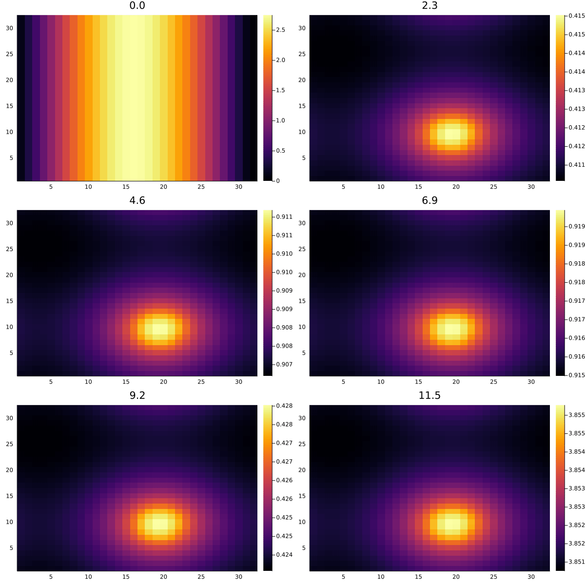

For v:

anim = @animate for k in 1:length(discrete_t)
    heatmap(solv[2:end, 2:end, k], title = "$(discrete_t[k])")
end
gif(anim, "Brusselator2Dsol_v.gif", fps = 8)