Schrödinger Equation

MethodOfLines can solve linear complex PDEs like the Schrödinger equation:

using MethodOfLines, OrdinaryDiffEq, Plots, DomainSets, ModelingToolkit

@parameters t, x
@variables ψ(..)::Complex

Dt = Differential(t)
Dxx = Differential(x)^2

xmin = 0
xmax = 1

V(x) = 0.0

eq = [im * Dt(ψ(t, x)) ~ Dxx(ψ(t, x)) + V(x) * ψ(t, x)] # You must enclose complex equations in a vector, even if there is only one equation

ψ0 = x -> ((1 + im)/sqrt(2))*sinpi(2*x)

bcs = [ψ(0, x) => ψ0(x), # Initial condition must be marked with a => operator
    ψ(t, xmin) ~ 0,
    ψ(t, xmax) ~ 0]

domains = [t ∈ Interval(0, 1), x ∈ Interval(xmin, xmax)]

@named sys = PDESystem(eq, bcs, domains, [t, x], [ψ(t, x)])

disc = MOLFiniteDifference([x => 100], t)

prob = discretize(sys, disc)

sol = solve(prob; saveat = 0.01)

discx = sol[x]
disct = sol[t]

discψ = sol[ψ(t, x)]
anim = @animate for i in 1:length(disct)
    u = discψ[i, :]
    plot(discx, [real.(u), imag.(u)], ylim = (-1.5, 1.5), title = "t = $(disct[i])",
        xlabel = "x", ylabel = "ψ(t,x)", label = ["re(ψ)" "im(ψ)"], legend = :topleft)
end
gif(anim, "schroedinger.gif", fps = 10)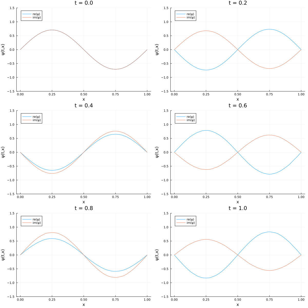

This linear Schrödinger equation works without a ::Complex annotation. For nonlinear PDE terms using conj, abs2, real, or imag, declare the field with ::Complex so Symbolics preserves those operations when constructing the PDE. Complex initial conditions must be marked with a => operator.

This represents the second from ground state of a particle in an infinite quantum well, try changing the potential V(x), initial conditions and BCs, it is extremely interesting to see how the wave function evolves even for nonphysical combinations. Be sure to post interesting results on the discourse!