Adding parameters

We can also build up more complicated systems with multiple dependent variables and parameters as follows

using ModelingToolkit, MethodOfLines, OrdinaryDiffEq, DomainSets

@parameters t x
@parameters Dn=0.5 Dp=2.0
@variables u(..) v(..)
Dt = Differential(t)
Dx = Differential(x)
Dxx = Differential(x)^2

eqs = [Dt(u(t, x)) ~ Dn * Dxx(u(t, x)) + u(t, x) * v(t, x),
    Dt(v(t, x)) ~ Dp * Dxx(v(t, x)) - u(t, x) * v(t, x)]
bcs = [u(0, x) ~ sin(pi * x / 2),
    v(0, x) ~ sin(pi * x / 2),
    u(t, 0) ~ 0.0, Dx(u(t, 1)) ~ 0.0,
    v(t, 0) ~ 0.0, Dx(v(t, 1)) ~ 0.0]

domains = [t ∈ Interval(0.0, 1.0),
    x ∈ Interval(0.0, 1.0)]

@named pdesys = PDESystem(
    eqs, bcs, domains, [t, x], [u(t, x), v(t, x)], [Dn, Dp])

discretization = MOLFiniteDifference([x => 0.1], t)

prob = discretize(pdesys, discretization) # This gives a DAEProblem since it's time-dependent

sol = solve(prob)

discrete_x = sol[x]
discrete_t = sol[t]

solu = sol[u(t, x)]
solv = sol[v(t, x)]

using Plots

anim = @animate for i in 1:length(discrete_t)
    p1 = plot(discrete_x, solu[i, :], label = "u, t=$(discrete_t[i])";
        legend = false, xlabel = "x", ylabel = "u", ylim = [0, 1])
    p2 = plot(discrete_x, solv[i, :], label = "v, t=$(discrete_t[i])";
        legend = false, xlabel = "x", ylabel = "v", ylim = [0, 1])
    plot(p1, p2)
end
gif(anim, "plot.gif", fps = 30)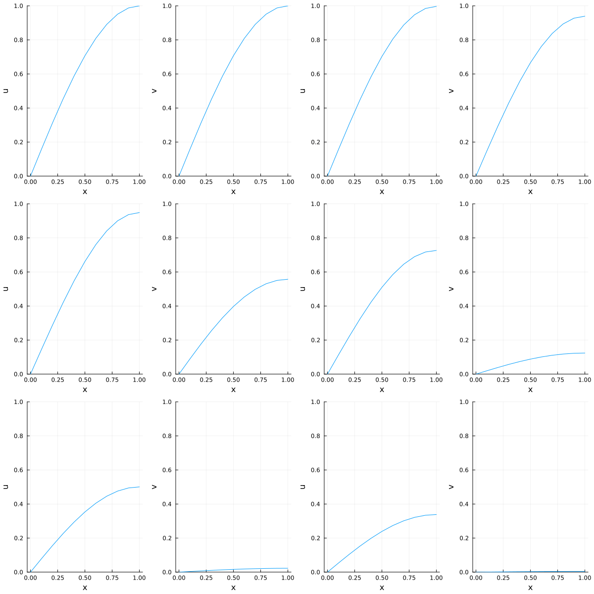

Remake with different parameter values

The system does not need to be re-discretized every time we want to plot with different parameters, the system can be remade with new parameters with remake. See the ModelingToolkit.jl docs for more ways to manipulate a prob post discretization.

using ModelingToolkit, MethodOfLines, OrdinaryDiffEq, DomainSets

@parameters t x
@parameters Dn=0.5 Dp=2.0
@variables u(..) v(..)
Dt = Differential(t)
Dx = Differential(x)
Dxx = Differential(x)^2

eqs = [Dt(u(t, x)) ~ Dn * Dxx(u(t, x)) + u(t, x) * v(t, x),
    Dt(v(t, x)) ~ Dp * Dxx(v(t, x)) - u(t, x) * v(t, x)]
bcs = [u(0, x) ~ sin(pi * x / 2),
    v(0, x) ~ sin(pi * x / 2),
    u(t, 0) ~ 0.0, Dx(u(t, 1)) ~ 0.0,
    v(t, 0) ~ 0.0, Dx(v(t, 1)) ~ 0.0]

domains = [t ∈ Interval(0.0, 1.0),
    x ∈ Interval(0.0, 1.0)]

@named pdesys = PDESystem(
    eqs, bcs, domains, [t, x], [u(t, x), v(t, x)], [Dn, Dp])

discretization = MOLFiniteDifference([x => 0.1], t)

prob = discretize(pdesys, discretization) # This gives a DAEProblem since it's time-dependent

sols = []
for (Dnval, Dpval) in zip(rand(10), rand(10))
    newprob = remake(prob, p = [Dn => Dnval, Dp => Dpval])
    push!(sols, solve(newprob))
end

using Plots
for (j, sol) in enumerate(sols)
    discrete_x = sol[x]
    discrete_t = sol[t]
    solu = sol[u(t, x)]
    solv = sol[v(t, x)]
    anim = @animate for i in 1:length(discrete_t)
        p1 = plot(discrete_x, solu[i, :], label = "u, t=$(discrete_t[i])";
            legend = false, xlabel = "x", ylabel = "u", ylim = [0, 1])
        p2 = plot(discrete_x, solv[i, :], label = "v, t=$(discrete_t[i])";
            legend = false, xlabel = "x", ylabel = "v", ylim = [0, 1])
        plot(p1, p2)
    end
    gif(anim, "plot_$j.gif", fps = 10)
end

[ Info: Saved animation to /home/runner/work/MethodOfLines.jl/MethodOfLines.jl/docs/build/tutorials/plot_1.gif
[ Info: Saved animation to /home/runner/work/MethodOfLines.jl/MethodOfLines.jl/docs/build/tutorials/plot_2.gif
[ Info: Saved animation to /home/runner/work/MethodOfLines.jl/MethodOfLines.jl/docs/build/tutorials/plot_3.gif
[ Info: Saved animation to /home/runner/work/MethodOfLines.jl/MethodOfLines.jl/docs/build/tutorials/plot_4.gif
[ Info: Saved animation to /home/runner/work/MethodOfLines.jl/MethodOfLines.jl/docs/build/tutorials/plot_5.gif
[ Info: Saved animation to /home/runner/work/MethodOfLines.jl/MethodOfLines.jl/docs/build/tutorials/plot_6.gif
[ Info: Saved animation to /home/runner/work/MethodOfLines.jl/MethodOfLines.jl/docs/build/tutorials/plot_7.gif
[ Info: Saved animation to /home/runner/work/MethodOfLines.jl/MethodOfLines.jl/docs/build/tutorials/plot_8.gif
[ Info: Saved animation to /home/runner/work/MethodOfLines.jl/MethodOfLines.jl/docs/build/tutorials/plot_9.gif
[ Info: Saved animation to /home/runner/work/MethodOfLines.jl/MethodOfLines.jl/docs/build/tutorials/plot_10.gif