Learning a missing term with a neural network

A neural network can stand in for a term of a PDE whose form is unknown and be trained on data. This is the universal differential equation (UDE) approach; the network comes from ModelingToolkitNeuralNets.jl. To MethodOfLines the network is a callable parameter of the PDESystem, so it is discretized like any other function of the field: with a scalar field input the interior of the equation stays a single array equation on the default DAEProblem path.

Data from a known model

The ground truth is the Fisher-KPP equation

\[\frac{\partial u}{\partial t} = D \frac{\partial^2 u}{\partial x^2} + u(1 - u), \qquad x \in [0, 1], \qquad u(t, 0) = u(t, 1) = 0.\]

We pretend the reaction term u(1 - u) is unknown and keep only the simulated data. The small initial condition and the long time span make the data cover u from 0 to about 0.9; the network can only be learned where the data constrains it.

using ModelingToolkit, MethodOfLines, OrdinaryDiffEq, DomainSets

@parameters t x
@variables u(..)
Dt = Differential(t)
Dxx = Differential(x)^2
D = 0.01

domains = [t ∈ Interval(0.0, 6.0), x ∈ Interval(0.0, 1.0)]
bcs = [u(0, x) ~ 0.1 * sinpi(x), u(t, 0) ~ 0.0, u(t, 1) ~ 0.0]
disc = MOLFiniteDifference([x => 0.05], t)

@named fisher = PDESystem(Dt(u(t, x)) ~ D * Dxx(u(t, x)) + u(t, x) * (1 - u(t, x)),
    bcs, domains, [t, x], [u(t, x)])

sol_true = solve(discretize(fisher, disc); saveat = 0.1)
data = sol_true[u(t, x)]
size(data)

(61, 21)

The UDE

SymbolicNeuralNetwork returns a symbolic callable NN and its parameter vector θ. NN(u(t, x), θ) is a vector with one entry, which replaces the reaction term. Both go into the parameter list of the PDESystem.

using ModelingToolkitNeuralNets

NN, θ = SymbolicNeuralNetwork(; n_input = 1, n_output = 1, nn_p_name = :θ)

@named ude = PDESystem(Dt(u(t, x)) ~ D * Dxx(u(t, x)) + NN(u(t, x), θ)[1],
    bcs, domains, [t, x], [u(t, x)], [NN, θ])

prob = discretize(ude, disc)

DAEProblem with uType Vector{Float64} and tType Float64. In-place: true
timespan: (0.0, 6.0)
u0: 21-element Vector{Float64}:
 0.0
 0.01564344650402309
 0.030901699437494747
 0.04539904997395468
 0.058778525229247314
 0.07071067811865475
 0.08090169943749474
 0.08910065241883679
 0.09510565162951537
 0.09876883405951378
 ⋮
 0.09510565162951537
 0.08910065241883679
 0.08090169943749476
 0.07071067811865475
 0.05877852522924731
 0.04539904997395469
 0.030901699437494736
 0.015643446504023103
 0.0
du0: 21-element Vector{Float64}:
 0.0
 0.0
 0.0
 0.0
 0.0
 0.0
 0.0
 0.0
 0.0
 0.0
 ⋮
 0.0
 0.0
 0.0
 0.0
 0.0
 0.0
 0.0
 0.0
 0.0

The network parameters are prob.ps[θ]. The default initialization keeps the network output near zero, so before training the UDE is plain diffusion.

Training

The loss simulates the UDE for a candidate θ and compares it with the data. setp_oop returns a function that builds a new parameter object from a vector, and remake puts it into the problem. Gradients come from ForwardDiff through the solve, which is cheap for a few dozen network parameters; the last section shows the reverse-mode alternative.

using Optimization, OptimizationOptimisers
using SymbolicIndexingInterface: setp_oop

set_θ = setp_oop(prob, θ)

function loss(ps, (prob, set_θ, data))
    newprob = remake(prob; p = set_θ(prob, ps))
    sol = solve(newprob; saveat = 0.1, verbose = DEVerbosity(SciMLLogging.None()))
    SciMLBase.successful_retcode(sol) || return Inf
    return sum(abs2, sol[u(t, x)] .- data)
end

optf = OptimizationFunction(loss, AutoForwardDiff())
optprob = OptimizationProblem(optf, collect(prob.ps[θ]), (prob, set_θ, data))
res = solve(optprob, Adam(0.02); maxiters = 2000)
res.objective

0.019997912855704555

The loss argument is called ps rather than x because x is the spatial variable used to index the solution.

Result

The fitted UDE against the data at a few times:

using Plots

sol_fit = solve(remake(prob; p = set_θ(prob, res.u)); saveat = 0.1)
fit = sol_fit[u(t, x)]
xs = sol_fit[x]
plt = plot(xlabel = "x", ylabel = "u")
for (k, i) in enumerate((1, 11, 21, 31, 61))
    plot!(plt, xs, data[i, :]; color = :black, label = k == 1 ? "data" : "")
    plot!(plt, xs, fit[i, :]; color = :red, linestyle = :dash, label = k == 1 ? "UDE" : "")
end
plt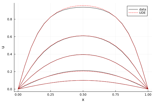

The learned term against the true one:

nn = prob.ps[NN]
us = range(0, 1; length = 50)
plot(us, us .* (1 .- us); label = "u(1 - u)", xlabel = "u", lw = 3)
plot!(us, [nn(ui, res.u)[1] for ui in us]; label = "NN(u)", lw = 3, linestyle = :dash)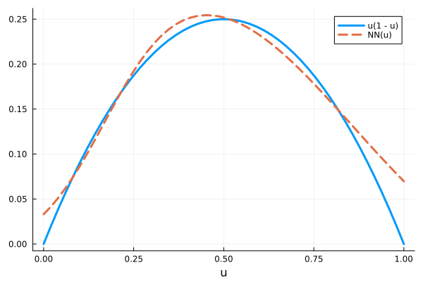

The network matches the true term where the data covers u and drifts near u = 0 and u = 1, where there is little data. Training takes a few minutes.

Adjoints

The same loss can be differentiated in reverse mode through SciMLSensitivity. Two things change: the solve gets wrap = Val(false), so the loss sees the solver's solution rather than the PDE wrapper, and the data enters as an array, since indexing a solution by u(t, x) has no reverse rule. Array(sol) holds the grid values with time along the second axis, the transpose of sol[u(t, x)].

using SciMLSensitivity, Zygote, ForwardDiff

function adjoint_loss(ps)
    newprob = remake(prob; p = set_θ(prob, ps))
    sol = solve(newprob; saveat = 0.1, wrap = Val(false),
        sensealg = InterpolatingAdjoint(autojacvec = ReverseDiffVJP(true)),
        abstol = 1.0e-8, reltol = 1.0e-8, verbose = DEVerbosity(SciMLLogging.None()))
    return sum(abs2, Array(sol) .- data')
end
g_adjoint = Zygote.gradient(adjoint_loss, res.u)[1]
g_forward = ForwardDiff.gradient(adjoint_loss, res.u)
maximum(abs.(g_adjoint .- g_forward)) / maximum(abs.(g_forward))

8.944548530153158e-7

AutoZygote() in place of AutoForwardDiff() trains with it. On this problem it is the slower tool: the adjoint solves a second DAE backwards in time for every gradient and takes two orders of magnitude longer than ForwardDiff, whose cost grows with the number of parameters instead. The balance tips only for much larger networks.

The Brusselator tutorial does the same with two fields as network input.