Diffusion Equation on a Square Plate

This tutorial considers a diffusion equation on a square plate:

\[\begin{equation*} \begin{aligned} \pdv{u(\vb x, t)}{t} &= \frac{1}{9}\grad^2 u(\vb x, t) & \vb x \in \Omega,\,t>0, \\[6pt] u(\vb x, t) & = 0 &\vb x \in \partial\Omega,\,t>0,\\[6pt] u(\vb x, 0) &= f(\vb x) & \vb x \in \Omega, \end{aligned} \end{equation*}\]

where $\Omega = [0, 2]^2$ and

\[f(x, y) = \begin{cases} 50 & y \leq 1, \\ 0 & y > 1. \end{cases}\]

To solve this problem, the first step is to define the mesh.

using FiniteVolumeMethod, DelaunayTriangulation
a, b, c, d = 0.0, 2.0, 0.0, 2.0
nx, ny = 50, 50
tri = triangulate_rectangle(a, b, c, d, nx, ny, single_boundary=true)
mesh = FVMGeometry(tri)

FVMGeometry with 2500 control volumes, 4802 triangles, and 7301 edges

This mesh is shown below.

using CairoMakie
fig, ax, sc = triplot(tri)
fig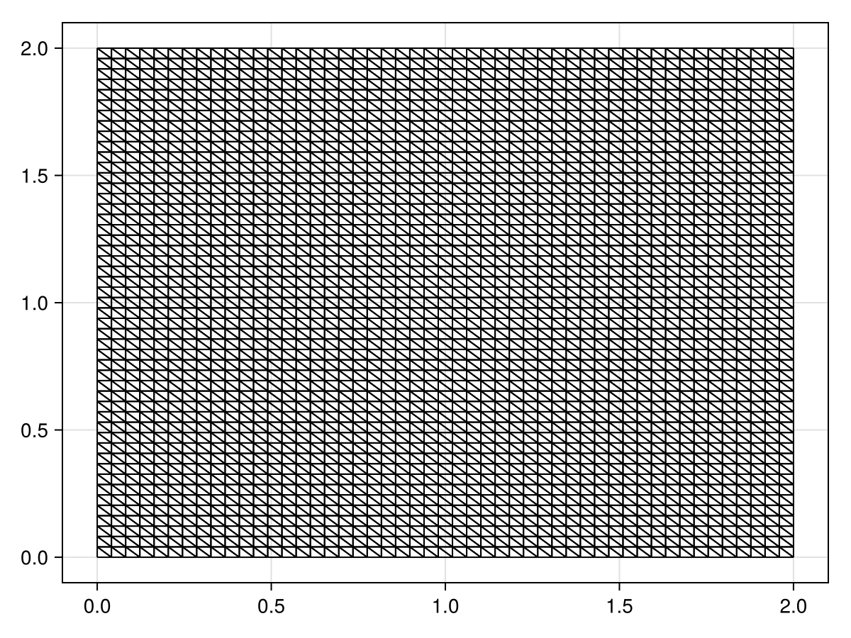

We now need to define the boundary conditions. We have a homogeneous Dirichlet condition:

bc = (x, y, t, u, p) -> zero(u)
BCs = BoundaryConditions(mesh, bc, Dirichlet)

BoundaryConditions with 1 boundary condition with type Dirichlet

We can now define the actual PDE. We start by defining the initial condition and the diffusion function.

f = (x, y) -> y ≤ 1.0 ? 50.0 : 0.0
initial_condition = [f(x, y) for (x, y) in DelaunayTriangulation.each_point(tri)]
D = (x, y, t, u, p) -> 1 / 9

#7 (generic function with 1 method)

We can now define the problem:

final_time = 0.5
prob = FVMProblem(mesh, BCs; diffusion_function=D, initial_condition, final_time)

FVMProblem with 2500 nodes and time span (0.0, 0.5)

Note that in prob, it is not a diffusion function that is used but instead it is a flux function:

prob.flux_function

#65 (generic function with 1 method)

When providing diffusion_function, the flux is given by $\vb q(\vb x, t, \alpha,\beta,\gamma) = (-\alpha/9, -\beta/9)^{\mkern-1.5mu\mathsf{T}}$, where $(\alpha, \beta, \gamma)$ defines the approximation to $u$ via $u(x, y) = \alpha x + \beta y + \gamma$ so that $\grad u(\vb x, t) = (\alpha,\beta)^{\mkern-1.5mu\mathsf{T}}$.

To now solve the problem, we simply use solve. Note that, in the solve call below, multithreading is enabled by default. (If you don't know what algorithm to consider, do using DifferentialEquations instead and simply call solve(prob, saveat=0.05) so that the algorithm is chosen automatically instead of using Tsit5().)

using OrdinaryDiffEq
sol = solve(prob, Tsit5(), saveat=0.05)

retcode: Success
Interpolation: 1st order linear
t: 11-element Vector{Float64}:
 0.0
 0.05
 0.1
 0.15
 0.2
 0.25
 0.3
 0.35
 0.4
 0.45
 0.5
u: 11-element Vector{Vector{Float64}}:
 [50.0, 50.0, 50.0, 50.0, 50.0, 50.0, 50.0, 50.0, 50.0, 50.0  …  0.0, 0.0, 0.0, 0.0, 0.0, 0.0, 0.0, 0.0, 0.0, 0.0]
 [0.0, 0.0, 0.0, 0.0, 0.0, 0.0, 0.0, 0.0, 0.0, 0.0  …  0.0, 0.0, 0.0, 0.0, 0.0, 0.0, 0.0, 0.0, 0.0, 0.0]
 [0.0, 0.0, 0.0, 0.0, 0.0, 0.0, 0.0, 0.0, 0.0, 0.0  …  0.0, 0.0, 0.0, 0.0, 0.0, 0.0, 0.0, 0.0, 0.0, 0.0]
 [0.0, 0.0, 0.0, 0.0, 0.0, 0.0, 0.0, 0.0, 0.0, 0.0  …  0.0, 0.0, 0.0, 0.0, 0.0, 0.0, 0.0, 0.0, 0.0, 0.0]
 [0.0, 0.0, 0.0, 0.0, 0.0, 0.0, 0.0, 0.0, 0.0, 0.0  …  0.0, 0.0, 0.0, 0.0, 0.0, 0.0, 0.0, 0.0, 0.0, 0.0]
 [0.0, 0.0, 0.0, 0.0, 0.0, 0.0, 0.0, 0.0, 0.0, 0.0  …  0.0, 0.0, 0.0, 0.0, 0.0, 0.0, 0.0, 0.0, 0.0, 0.0]
 [0.0, 0.0, 0.0, 0.0, 0.0, 0.0, 0.0, 0.0, 0.0, 0.0  …  0.0, 0.0, 0.0, 0.0, 0.0, 0.0, 0.0, 0.0, 0.0, 0.0]
 [0.0, 0.0, 0.0, 0.0, 0.0, 0.0, 0.0, 0.0, 0.0, 0.0  …  0.0, 0.0, 0.0, 0.0, 0.0, 0.0, 0.0, 0.0, 0.0, 0.0]
 [0.0, 0.0, 0.0, 0.0, 0.0, 0.0, 0.0, 0.0, 0.0, 0.0  …  0.0, 0.0, 0.0, 0.0, 0.0, 0.0, 0.0, 0.0, 0.0, 0.0]
 [0.0, 0.0, 0.0, 0.0, 0.0, 0.0, 0.0, 0.0, 0.0, 0.0  …  0.0, 0.0, 0.0, 0.0, 0.0, 0.0, 0.0, 0.0, 0.0, 0.0]
 [0.0, 0.0, 0.0, 0.0, 0.0, 0.0, 0.0, 0.0, 0.0, 0.0  …  0.0, 0.0, 0.0, 0.0, 0.0, 0.0, 0.0, 0.0, 0.0, 0.0]

To visualise the solution, we can use tricontourf! from Makie.jl.

fig = Figure(fontsize=38)
for (i, j) in zip(1:3, (1, 6, 11))
    local ax
    ax = Axis(fig[1, i], width=600, height=600,
        xlabel="x", ylabel="y",
        title="t = $(sol.t[j])",
        titlealign=:left)
    tricontourf!(ax, tri, sol.u[j], levels=0:5:50, colormap=:matter)
    tightlimits!(ax)
end
resize_to_layout!(fig)
fig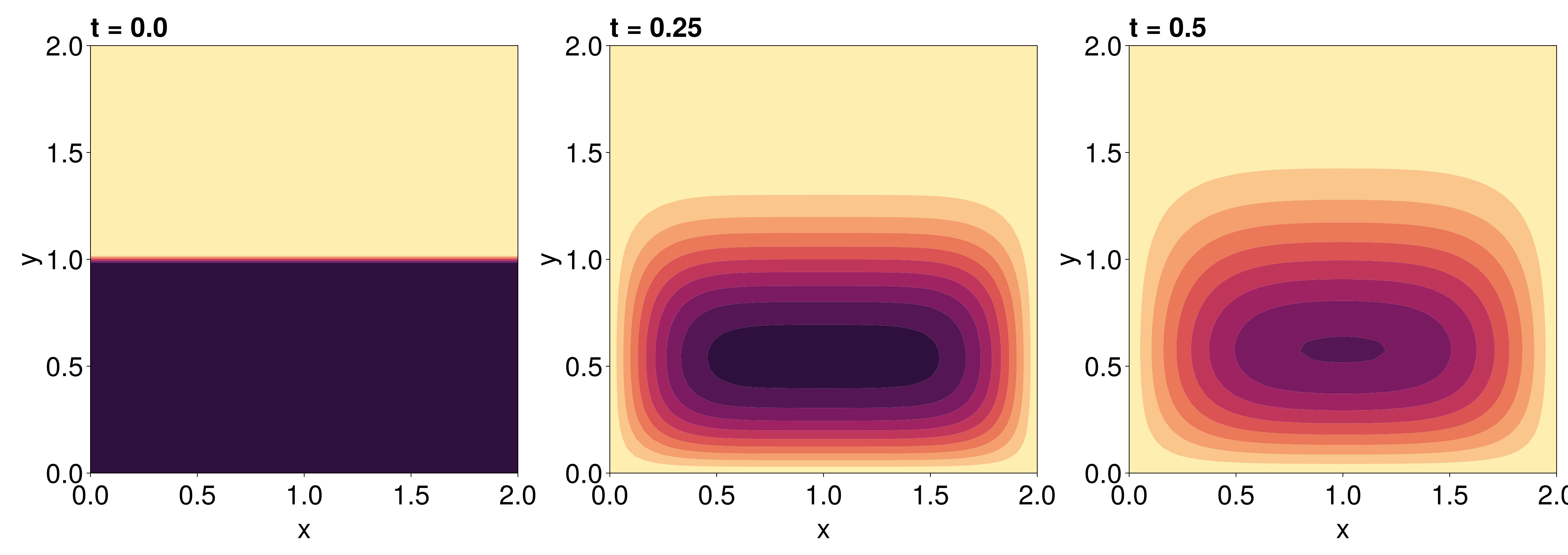

    local ax

Just the code

An uncommented version of this example is given below. You can view the source code for this file here.

using FiniteVolumeMethod, DelaunayTriangulation
a, b, c, d = 0.0, 2.0, 0.0, 2.0
nx, ny = 50, 50
tri = triangulate_rectangle(a, b, c, d, nx, ny, single_boundary=true)
mesh = FVMGeometry(tri)

using CairoMakie
fig, ax, sc = triplot(tri)
fig

bc = (x, y, t, u, p) -> zero(u)
BCs = BoundaryConditions(mesh, bc, Dirichlet)

f = (x, y) -> y ≤ 1.0 ? 50.0 : 0.0
initial_condition = [f(x, y) for (x, y) in DelaunayTriangulation.each_point(tri)]
D = (x, y, t, u, p) -> 1 / 9

final_time = 0.5
prob = FVMProblem(mesh, BCs; diffusion_function=D, initial_condition, final_time)

prob.flux_function

using OrdinaryDiffEq
sol = solve(prob, Tsit5(), saveat=0.05)

fig = Figure(fontsize=38)
for (i, j) in zip(1:3, (1, 6, 11))
    local ax
    ax = Axis(fig[1, i], width=600, height=600,
        xlabel="x", ylabel="y",
        title="t = $(sol.t[j])",
        titlealign=:left)
    tricontourf!(ax, tri, sol.u[j], levels=0:5:50, colormap=:matter)
    tightlimits!(ax)
end
resize_to_layout!(fig)
fig

    local ax

This page was generated using Literate.jl.