Porous-Fisher Equation and Travelling Waves

This tutorial considers a more involved example, where we discuss travelling wave solutions of a Porous-Fisher equation:

\[\begin{equation*} \begin{aligned} \pdv{u(\vb x, t)}{t} &= D \div[u\grad u] + \lambda u(1-u) & 0<x<a,\,0<y<b,\,t>0,\\[6pt] u(x, 0, t) & = 1 & 0<x<a,\,t>0,\\[6pt] u(x, b, t) & = 0 & 0<x<a,\,t>0,\\[6pt] \pdv{u(0, y, t)}{x} &= 0 & 0<y<b,\,t>0,\\[6pt] \pdv{u(a, y, t)}{x} &= 0 & 0 < y < b,\,t>0,\\[6pt] u(\vb x, 0) & = f(y) & 0 \leq x \leq a,\, 0 \leq y\leq b. \end{aligned} \end{equation*}\]

This problem is defined on the rectangle $[0, a] \times [0, b]$ and we assume that $b \gg a$ so that the rectangle is much taller than it is wide. This problem has $u$ ranging from $u=1$ at the bottom of the rectangle down to $u=0$ at the top on the rectangle, and with zero flux conditions on the two vertical walls. We take the initial condition $f$ to be independent of $x$. This setup implies that the solution along each constant line $x=x_0$ should be about the same, i.e. the problem is invariant in $x$. If indeed we have $u(\vb x, t) = u(y, t)$ then the PDE becomes

\[\begin{equation}\label{eq:onedproblem} \pdv{u(y, t)}{t} = D\pdv{y}\left(u\pdv{u}{y}\right) + \lambda u(1-u), \end{equation}\]

which has travelling wave solutions. Following the analysis given in Section 13.4 of the book Mathematical biology I: An introduction by J. D. Murray (2002), we can show that a travelling wave solution to the one-dimensional problem \eqref{eq:onedproblem} is given by

\[\begin{equation}\label{eq:onedproblemexact} u(y, t) = \begin{cases} 1-\mathrm{e}^{c_{\min}z} & z \leq 0, \\ 0 & z > 0, \end{cases} \end{equation}\]

where $c_{\min} = \sqrt{\lambda/(2D)}$, $c = \sqrt{D\lambda/2}$, and $z = x-ct$ is the travelling wave coordinates. This travelling wave would mathc our problem exactly if the rectangle were instead $[0, a] \times \mathbb R$, but by choosing $b$ large enough we can at least emulate the travelling wave behaviour closely; the homogeneous Neumann conditions are to ensure no energy is lost, thus allowing the travelling waves to exist. Moreover, note that the approximations of the solution with $u(y, t)$ in \eqref{eq:onedproblemexact} will only be accurate for large time as it takes the solution some time to evolve towards the travelling wave solution.

Now with this preamble out of the way, let us solve this problem.

using DelaunayTriangulation, FiniteVolumeMethod, OrdinaryDiffEq, LinearSolve
a, b, c, d, nx, ny = 0.0, 3.0, 0.0, 40.0, 60, 80
tri = triangulate_rectangle(a, b, c, d, nx, ny; single_boundary=false)
mesh = FVMGeometry(tri)
one_bc = (x, y, t, u, p) -> one(u)
zero_bc = (x, y, t, u, p) -> zero(u)
bc_fncs = (one_bc, zero_bc, zero_bc, zero_bc) # bottom, right, top, left
types = (Dirichlet, Neumann, Dirichlet, Neumann)
BCs = BoundaryConditions(mesh, bc_fncs, types)
f = (x, y) -> zero(y)
diffusion_function = (x, y, t, u, D) -> D * u
source_function = (x, y, t, u, λ) -> λ * u * (1 - u)
D, λ = 0.9, 0.99
diffusion_parameters = D
source_parameters = λ
final_time = 50.0
initial_condition = [f(x, y) for (x, y) in DelaunayTriangulation.each_point(tri)]
prob = FVMProblem(mesh, BCs;
    diffusion_function, diffusion_parameters,
    source_function, source_parameters,
    initial_condition, final_time)
sol = solve(prob, TRBDF2(linsolve=KLUFactorization()); saveat=0.5)

retcode: Success
Interpolation: 1st order linear
t: 101-element Vector{Float64}:
  0.0
  0.5
  1.0
  1.5
  2.0
  ⋮
 48.0
 48.5
 49.0
 49.5
 50.0
u: 101-element Vector{Vector{Float64}}:
 [0.0, 0.0, 0.0, 0.0, 0.0, 0.0, 0.0, 0.0, 0.0, 0.0  …  0.0, 0.0, 0.0, 0.0, 0.0, 0.0, 0.0, 0.0, 0.0, 0.0]
 [1.0, 1.0, 1.0, 1.0, 1.0, 1.0, 1.0, 1.0, 1.0, 1.0  …  0.0, 0.0, 0.0, 0.0, 0.0, 0.0, 0.0, 0.0, 0.0, 0.0]
 [1.0, 1.0, 1.0, 1.0, 1.0, 1.0, 1.0, 1.0, 1.0, 1.0  …  0.0, 0.0, 0.0, 0.0, 0.0, 0.0, 0.0, 0.0, 0.0, 0.0]
 [1.0, 1.0, 1.0, 1.0, 1.0, 1.0, 1.0, 1.0, 1.0, 1.0  …  0.0, 0.0, 0.0, 0.0, 0.0, 0.0, 0.0, 0.0, 0.0, 0.0]
 [1.0, 1.0, 1.0, 1.0, 1.0, 1.0, 1.0, 1.0, 1.0, 1.0  …  0.0, 0.0, 0.0, 0.0, 0.0, 0.0, 0.0, 0.0, 0.0, 0.0]
 ⋮
 [1.0, 1.0, 1.0, 1.0, 1.0, 1.0, 1.0, 1.0, 1.0, 1.0  …  0.0, 0.0, 0.0, 0.0, 0.0, 0.0, 0.0, 0.0, 0.0, 0.0]
 [1.0, 1.0, 1.0, 1.0, 1.0, 1.0, 1.0, 1.0, 1.0, 1.0  …  0.0, 0.0, 0.0, 0.0, 0.0, 0.0, 0.0, 0.0, 0.0, 0.0]
 [1.0, 1.0, 1.0, 1.0, 1.0, 1.0, 1.0, 1.0, 1.0, 1.0  …  0.0, 0.0, 0.0, 0.0, 0.0, 0.0, 0.0, 0.0, 0.0, 0.0]
 [1.0, 1.0, 1.0, 1.0, 1.0, 1.0, 1.0, 1.0, 1.0, 1.0  …  0.0, 0.0, 0.0, 0.0, 0.0, 0.0, 0.0, 0.0, 0.0, 0.0]
 [1.0, 1.0, 1.0, 1.0, 1.0, 1.0, 1.0, 1.0, 1.0, 1.0  …  0.0, 0.0, 0.0, 0.0, 0.0, 0.0, 0.0, 0.0, 0.0, 0.0]

Let us now look at the travelling wave behaviour. We will plot the evolution over time, and also the travelling wave view of the solution. First, let us get these travelling wave values.

large_time_idx = findfirst(≥(10.0), sol.t)
c = sqrt(λ / (2D))
cₘᵢₙ = sqrt(λ * D / 2)
zᶜ = 0.0
exact_solution(z) = ifelse(z ≤ zᶜ, 1 - exp(cₘᵢₙ * z), zero(z))
travelling_wave_values = zeros(ny, length(sol) - large_time_idx + 1)
z_vals = zero(travelling_wave_values)
u_mat = [reshape(u, (nx, ny)) for u in sol.u]
for (i, t_idx) in pairs(large_time_idx:lastindex(sol))
    u = u_mat[t_idx]
    τ = sol.t[t_idx]
    for k in 1:ny
        y = c + (k - 1) * (d - c) / (ny - 1)
        z = y - c * τ
        z_vals[k, i] = z
        travelling_wave_values[k, i] = u[nx÷2, k]
    end
end

Now we are in a position to plot.

using CairoMakie
fig = Figure(resolution=(3200.72f0, 800.64f0), fontsize=38)
for (i, j) in zip(1:3, (1, 51, 101))
    ax = Axis(fig[1, i], width=600, height=600,
        xlabel="x", ylabel="y",
        title="t = $(sol.t[j])",
        titlealign=:left)
    tricontourf!(ax, tri, sol.u[j], levels=0:0.05:1, colormap=:matter)
    tightlimits!(ax)
end
ax = Axis(fig[1, 4], width=900, height=600)
colors = cgrad(:matter, length(sol) - large_time_idx + 1; categorical=false)
[lines!(ax, z_vals[:, i], travelling_wave_values[:, i], color=colors[i], linewidth=2) for i in 1:(length(sol)-large_time_idx+1)]
exact_z_vals = collect(LinRange(extrema(z_vals)..., 500))
exact_travelling_wave_values = exact_solution.(exact_z_vals)
lines!(ax, exact_z_vals, exact_travelling_wave_values, color=:red, linewidth=4, linestyle=:dash)
fig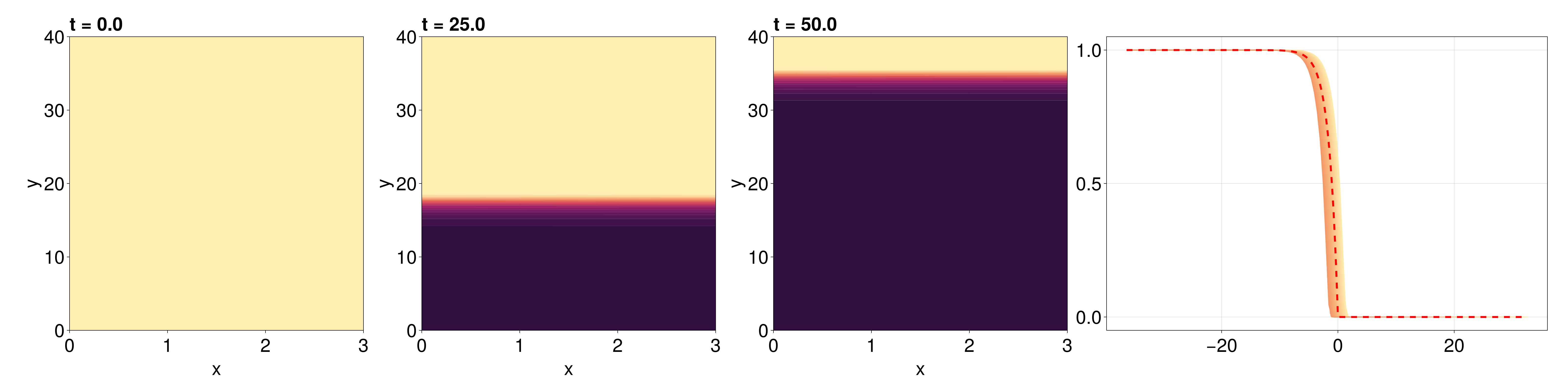

Just the code

An uncommented version of this example is given below. You can view the source code for this file here.

using DelaunayTriangulation, FiniteVolumeMethod, OrdinaryDiffEq, LinearSolve
a, b, c, d, nx, ny = 0.0, 3.0, 0.0, 40.0, 60, 80
tri = triangulate_rectangle(a, b, c, d, nx, ny; single_boundary=false)
mesh = FVMGeometry(tri)
one_bc = (x, y, t, u, p) -> one(u)
zero_bc = (x, y, t, u, p) -> zero(u)
bc_fncs = (one_bc, zero_bc, zero_bc, zero_bc) # bottom, right, top, left
types = (Dirichlet, Neumann, Dirichlet, Neumann)
BCs = BoundaryConditions(mesh, bc_fncs, types)
f = (x, y) -> zero(y)
diffusion_function = (x, y, t, u, D) -> D * u
source_function = (x, y, t, u, λ) -> λ * u * (1 - u)
D, λ = 0.9, 0.99
diffusion_parameters = D
source_parameters = λ
final_time = 50.0
initial_condition = [f(x, y) for (x, y) in DelaunayTriangulation.each_point(tri)]
prob = FVMProblem(mesh, BCs;
    diffusion_function, diffusion_parameters,
    source_function, source_parameters,
    initial_condition, final_time)
sol = solve(prob, TRBDF2(linsolve=KLUFactorization()); saveat=0.5)

large_time_idx = findfirst(≥(10.0), sol.t)
c = sqrt(λ / (2D))
cₘᵢₙ = sqrt(λ * D / 2)
zᶜ = 0.0
exact_solution(z) = ifelse(z ≤ zᶜ, 1 - exp(cₘᵢₙ * z), zero(z))
travelling_wave_values = zeros(ny, length(sol) - large_time_idx + 1)
z_vals = zero(travelling_wave_values)
u_mat = [reshape(u, (nx, ny)) for u in sol.u]
for (i, t_idx) in pairs(large_time_idx:lastindex(sol))
    u = u_mat[t_idx]
    τ = sol.t[t_idx]
    for k in 1:ny
        y = c + (k - 1) * (d - c) / (ny - 1)
        z = y - c * τ
        z_vals[k, i] = z
        travelling_wave_values[k, i] = u[nx÷2, k]
    end
end

using CairoMakie
fig = Figure(resolution=(3200.72f0, 800.64f0), fontsize=38)
for (i, j) in zip(1:3, (1, 51, 101))
    ax = Axis(fig[1, i], width=600, height=600,
        xlabel="x", ylabel="y",
        title="t = $(sol.t[j])",
        titlealign=:left)
    tricontourf!(ax, tri, sol.u[j], levels=0:0.05:1, colormap=:matter)
    tightlimits!(ax)
end
ax = Axis(fig[1, 4], width=900, height=600)
colors = cgrad(:matter, length(sol) - large_time_idx + 1; categorical=false)
[lines!(ax, z_vals[:, i], travelling_wave_values[:, i], color=colors[i], linewidth=2) for i in 1:(length(sol)-large_time_idx+1)]
exact_z_vals = collect(LinRange(extrema(z_vals)..., 500))
exact_travelling_wave_values = exact_solution.(exact_z_vals)
lines!(ax, exact_z_vals, exact_travelling_wave_values, color=:red, linewidth=4, linestyle=:dash)
fig

This page was generated using Literate.jl.