Porous-Medium Equation
No source
In this tutorial, we consider the porous-medium equation, given by
\[\pdv{u}{t} = D\div[u^{m-1}\grad u],\]
with initial condition $u(\vb x, 0) = M\delta(\vb x)$ where $\delta(\vb x)$ is the Dirac delta function and $M = \iint_{\mathbb R^2} u(\vb x, t) \dd{A}$. The diffusion function for this problem is $D(\vb x, t, u) = Du^{m-1}$. To approximate $\delta(\vb x)$, we use
\[\delta(\vb x) \approx g(\vb x) = \frac{1}{\varepsilon^2\pi}\exp\left[-\frac{1}{\varepsilon^2}\left(x^2 + y^2\right)\right],\]
taking $\varepsilon = 0.1$. It can be shown[1] that $u(\vb x, t)$ is zero for $x^2 + y^2 \geq R_{m, M}(Dt)^{1/m}$, where
\[R_{m, M} = \left(\frac{4m}{m-1}\right)\left[\frac{M}{4\pi}\right]^{(m-1)/m},\]
so we can replace the domain $\mathbb R^2$ with the domain $\Omega = [-L, L]^2$ where $L = R_{m, M}^{1/2}(DT)^{1/2m}$ and $T$ is the time that we solve up. We use a Dirichlet boundary condition on $\partial\Omega$.
Let us now solve this problem, taking $m = 2$, $M = 0.37$, $D = 2.53$, and $T = 12$.
using DelaunayTriangulation, FiniteVolumeMethod

# Step 0: Define all the parameters
m = 2
M = 0.37
D = 2.53
final_time = 12.0
ε = 0.1
# Step 1: Define the mesh
RmM = 4m / (m - 1) * (M / (4π))^((m - 1) / m)
L = sqrt(RmM) * (D * final_time)^(1 / (2m))
tri = triangulate_rectangle(-L, L, -L, L, 125, 125, single_boundary=true)
mesh = FVMGeometry(tri)
FVMGeometry with 15625 control volumes, 30752 triangles, and 46376 edges# Step 2: Define the boundary conditions
BCs = BoundaryConditions(mesh, (x, y, t, u, p) -> zero(u), Dirichlet)BoundaryConditions with 1 boundary condition with type Dirichlet# Step 3: Define the actual PDE
f = (x, y) -> M * 1 / (ε^2 * π) * exp(-1 / (ε^2) * (x^2 + y^2))
diffusion_function = (x, y, t, u, p) -> p[1] * u^(p[2] - 1)
diffusion_parameters = (D, m)
initial_condition = [f(x, y) for (x, y) in DelaunayTriangulation.each_point(tri)]
prob = FVMProblem(mesh, BCs;
diffusion_function,
diffusion_parameters,
initial_condition,
final_time)FVMProblem with 15625 nodes and time span (0.0, 12.0)# Step 4: Solve
using LinearSolve, OrdinaryDiffEq
sol = solve(prob, TRBDF2(linsolve=KLUFactorization()); saveat=3.0)retcode: Success
Interpolation: 1st order linear
t: 5-element Vector{Float64}:
0.0
3.0
6.0
9.0
12.0
u: 5-element Vector{Vector{Float64}}:
[0.0, 0.0, 0.0, 0.0, 0.0, 0.0, 0.0, 0.0, 0.0, 0.0 … 0.0, 0.0, 0.0, 0.0, 0.0, 0.0, 0.0, 0.0, 0.0, 0.0]
[0.0, 0.0, 0.0, 0.0, 0.0, 0.0, 0.0, 0.0, 0.0, 0.0 … 0.0, 0.0, 0.0, 0.0, 0.0, 0.0, 0.0, 0.0, 0.0, 0.0]
[0.0, 0.0, 0.0, 0.0, 0.0, 0.0, 0.0, 0.0, 0.0, 0.0 … 0.0, 0.0, 0.0, 0.0, 0.0, 0.0, 0.0, 0.0, 0.0, 0.0]
[0.0, 0.0, 0.0, 0.0, 0.0, 0.0, 0.0, 0.0, 0.0, 0.0 … 0.0, 0.0, 0.0, 0.0, 0.0, 0.0, 0.0, 0.0, 0.0, 0.0]
[0.0, 0.0, 0.0, 0.0, 0.0, 0.0, 0.0, 0.0, 0.0, 0.0 … 0.0, 0.0, 0.0, 0.0, 0.0, 0.0, 0.0, 0.0, 0.0, 0.0]# Step 5: Visualise
using CairoMakie
fig = Figure(fontsize=38)
for (i, j) in zip(1:3, (1, 3, 5))
ax = Axis(fig[1, i], width=600, height=600,
xlabel="x", ylabel="y",
title="t = $(sol.t[j])",
titlealign=:left)
tricontourf!(ax, tri, sol.u[j], levels=0:0.005:0.05, colormap=:matter, extendhigh=:auto)
tightlimits!(ax)
end
resize_to_layout!(fig)
fig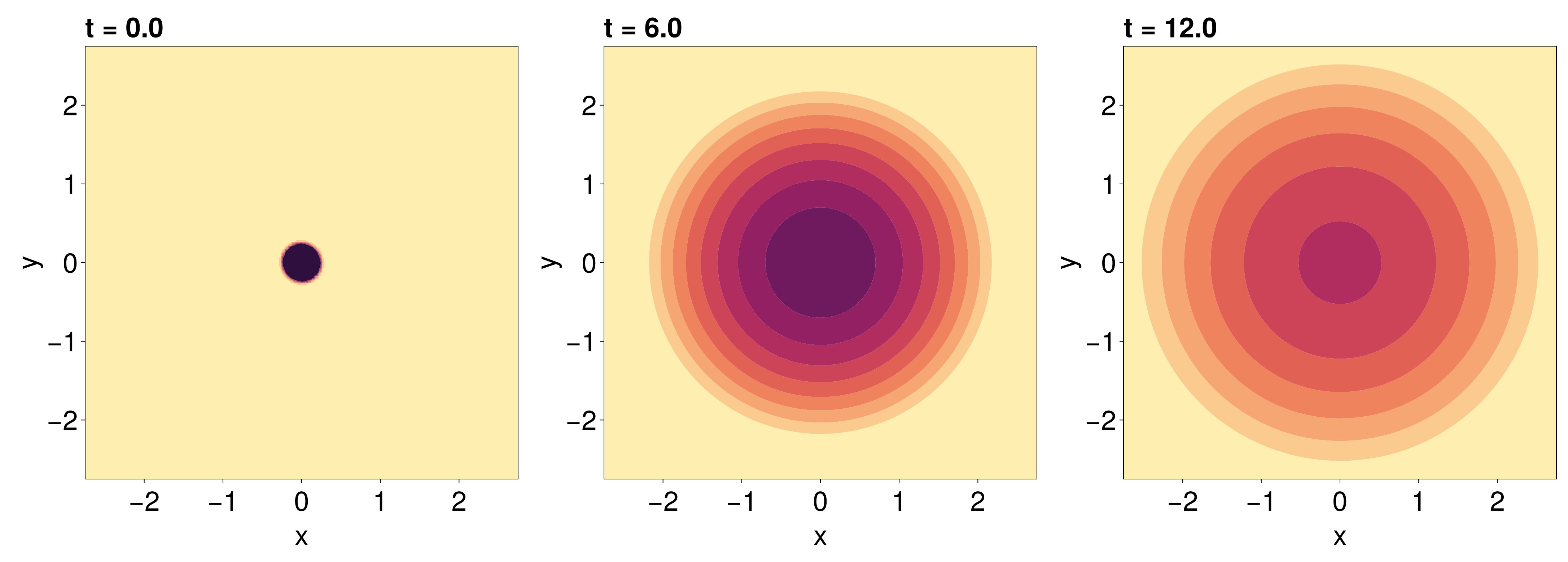
Linear source
Let us now extend the problem above so that a linear source is now included:
\[\pdv{u}{t} = D\div [u^{m-1}\grad u] + \lambda u, \quad \lambda > 0.\]
We again let the initial condition be $u(\vb x, 0) = M\delta(\vb x)$. For the domain, we use
\[\Omega = \left[-R_{m, M}^{1/2}\tau(T)^{1/2m}, R_{m,M}^{1/2}\tau(T)^{1/2m}\right]^2,\]
where
\[\tau(T) = \frac{D}{\lambda(m-1)}\left[\mathrm{e}^{\lambda(m-1)T}-1\right].\]
The code below solves this problem.
# Step 0: Define all the parameters
m = 3.4
M = 2.3
D = 0.581
λ = 0.2
final_time = 10.0
ε = 0.1
# Step 1: Define the mesh
RmM = 4m / (m - 1) * (M / (4π))^((m - 1) / m)
L = sqrt(RmM) * (D / (λ * (m - 1)) * (exp(λ * (m - 1) * final_time) - 1))^(1 / (2m))
tri = triangulate_rectangle(-L, L, -L, L, 125, 125, single_boundary=true)
mesh = FVMGeometry(tri)FVMGeometry with 15625 control volumes, 30752 triangles, and 46376 edges# Step 2: Define the boundary conditions
bc = (x, y, t, u, p) -> zero(u)
type = Dirichlet
BCs = BoundaryConditions(mesh, bc, type)BoundaryConditions with 1 boundary condition with type Dirichlet# Step 3: Define the actual PDE
f = (x, y) -> M * 1 / (ε^2 * π) * exp(-1 / (ε^2) * (x^2 + y^2))
diffusion_function = (x, y, t, u, p) -> p.D * abs(u)^(p.m - 1)
source_function = (x, y, t, u, λ) -> λ * u
diffusion_parameters = (D=D, m=m)
source_parameters = λ
initial_condition = [f(x, y) for (x, y) in DelaunayTriangulation.each_point(tri)]
prob = FVMProblem(mesh, BCs;
diffusion_function,
diffusion_parameters,
source_function,
source_parameters,
initial_condition,
final_time)FVMProblem with 15625 nodes and time span (0.0, 10.0)# Step 4: Solve
sol = solve(prob, TRBDF2(linsolve=KLUFactorization()); saveat=2.5)retcode: Success
Interpolation: 1st order linear
t: 5-element Vector{Float64}:
0.0
2.5
5.0
7.5
10.0
u: 5-element Vector{Vector{Float64}}:
[0.0, 0.0, 0.0, 0.0, 0.0, 0.0, 0.0, 0.0, 0.0, 0.0 … 0.0, 0.0, 0.0, 0.0, 0.0, 0.0, 0.0, 0.0, 0.0, 0.0]
[0.0, 0.0, 0.0, 0.0, 0.0, 0.0, 0.0, 0.0, 0.0, 0.0 … 0.0, 0.0, 0.0, 0.0, 0.0, 0.0, 0.0, 0.0, 0.0, 0.0]
[0.0, 0.0, 0.0, 0.0, 0.0, 0.0, 0.0, 0.0, 0.0, 0.0 … 0.0, 0.0, 0.0, 0.0, 0.0, 0.0, 0.0, 0.0, 0.0, 0.0]
[0.0, 0.0, 0.0, 0.0, 0.0, 0.0, 0.0, 0.0, 0.0, 0.0 … 0.0, 0.0, 0.0, 0.0, 0.0, 0.0, 0.0, 0.0, 0.0, 0.0]
[0.0, 0.0, 0.0, 0.0, 0.0, 0.0, 0.0, 0.0, 0.0, 0.0 … 0.0, 0.0, 0.0, 0.0, 0.0, 0.0, 0.0, 0.0, 0.0, 0.0]# Step 5: Visualise
fig = Figure(fontsize=38)
for (i, j) in zip(1:3, (1, 3, 5))
ax = Axis(fig[1, i], width=600, height=600,
xlabel="x", ylabel="y",
title="t = $(sol.t[j])",
titlealign=:left)
tricontourf!(ax, tri, sol.u[j], levels=0:0.05:1, extendlow=:auto, colormap=:matter, extendhigh=:auto)
tightlimits!(ax)
end
resize_to_layout!(fig)
fig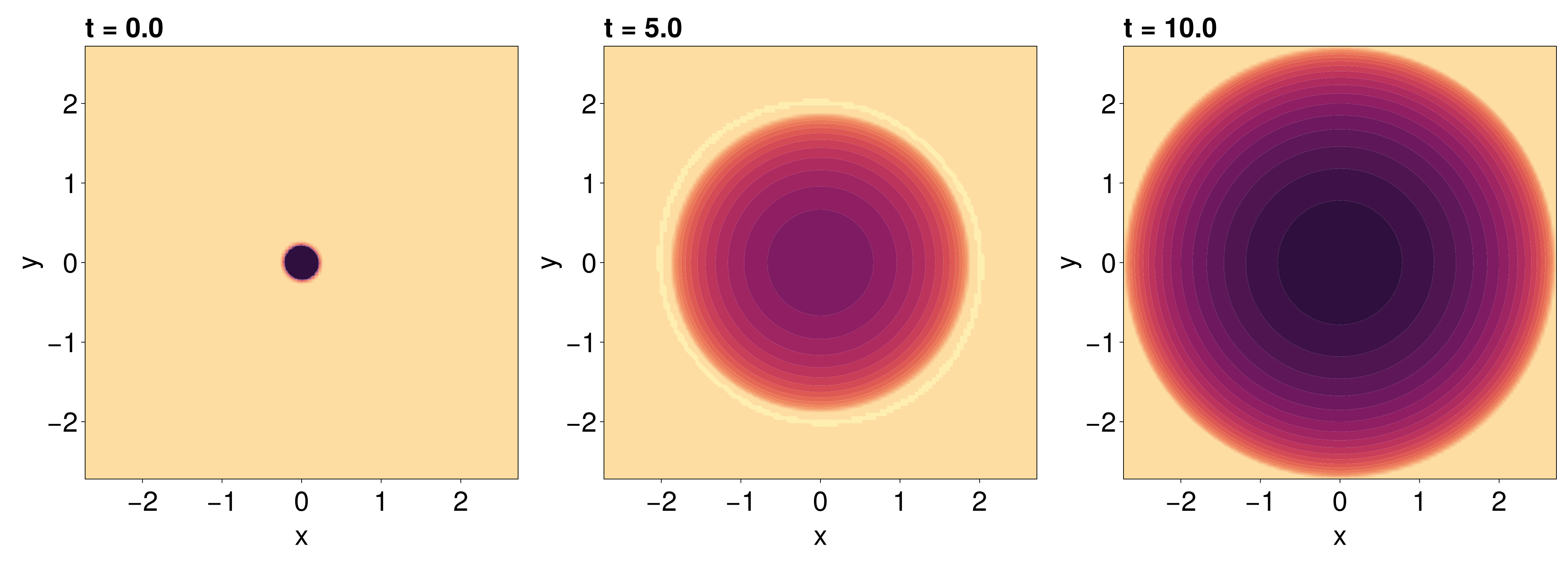
Just the code
An uncommented version of this example is given below. You can view the source code for this file here.
using DelaunayTriangulation, FiniteVolumeMethod
# Step 0: Define all the parameters
m = 2
M = 0.37
D = 2.53
final_time = 12.0
ε = 0.1
# Step 1: Define the mesh
RmM = 4m / (m - 1) * (M / (4π))^((m - 1) / m)
L = sqrt(RmM) * (D * final_time)^(1 / (2m))
tri = triangulate_rectangle(-L, L, -L, L, 125, 125, single_boundary=true)
mesh = FVMGeometry(tri)
# Step 2: Define the boundary conditions
BCs = BoundaryConditions(mesh, (x, y, t, u, p) -> zero(u), Dirichlet)
# Step 3: Define the actual PDE
f = (x, y) -> M * 1 / (ε^2 * π) * exp(-1 / (ε^2) * (x^2 + y^2))
diffusion_function = (x, y, t, u, p) -> p[1] * u^(p[2] - 1)
diffusion_parameters = (D, m)
initial_condition = [f(x, y) for (x, y) in DelaunayTriangulation.each_point(tri)]
prob = FVMProblem(mesh, BCs;
    diffusion_function,
    diffusion_parameters,
    initial_condition,
    final_time)
# Step 4: Solve
using LinearSolve, OrdinaryDiffEq
sol = solve(prob, TRBDF2(linsolve=KLUFactorization()); saveat=3.0)
# Step 5: Visualise
using CairoMakie
fig = Figure(fontsize=38)
for (i, j) in zip(1:3, (1, 3, 5))
    ax = Axis(fig[1, i], width=600, height=600,
        xlabel="x", ylabel="y",
        title="t = $(sol.t[j])",
        titlealign=:left)
    tricontourf!(ax, tri, sol.u[j], levels=0:0.005:0.05, colormap=:matter, extendhigh=:auto)
    tightlimits!(ax)
end
resize_to_layout!(fig)
fig
# Step 0: Define all the parameters
m = 3.4
M = 2.3
D = 0.581
λ = 0.2
final_time = 10.0
ε = 0.1
# Step 1: Define the mesh
RmM = 4m / (m - 1) * (M / (4π))^((m - 1) / m)
L = sqrt(RmM) * (D / (λ * (m - 1)) * (exp(λ * (m - 1) * final_time) - 1))^(1 / (2m))
tri = triangulate_rectangle(-L, L, -L, L, 125, 125, single_boundary=true)
mesh = FVMGeometry(tri)
# Step 2: Define the boundary conditions
bc = (x, y, t, u, p) -> zero(u)
type = Dirichlet
BCs = BoundaryConditions(mesh, bc, type)
# Step 3: Define the actual PDE
f = (x, y) -> M * 1 / (ε^2 * π) * exp(-1 / (ε^2) * (x^2 + y^2))
diffusion_function = (x, y, t, u, p) -> p.D * abs(u)^(p.m - 1)
source_function = (x, y, t, u, λ) -> λ * u
diffusion_parameters = (D=D, m=m)
source_parameters = λ
initial_condition = [f(x, y) for (x, y) in DelaunayTriangulation.each_point(tri)]
prob = FVMProblem(mesh, BCs;
    diffusion_function,
    diffusion_parameters,
    source_function,
    source_parameters,
    initial_condition,
    final_time)
# Step 4: Solve
sol = solve(prob, TRBDF2(linsolve=KLUFactorization()); saveat=2.5)
# Step 5: Visualise
fig = Figure(fontsize=38)
for (i, j) in zip(1:3, (1, 3, 5))
    ax = Axis(fig[1, i], width=600, height=600,
        xlabel="x", ylabel="y",
        title="t = $(sol.t[j])",
        titlealign=:left)
    tricontourf!(ax, tri, sol.u[j], levels=0:0.05:1, extendlow=:auto, colormap=:matter, extendhigh=:auto)
    tightlimits!(ax)
end
resize_to_layout!(fig)
figThis page was generated using Literate.jl.