Mean Exit Time Problems

• Mean Exit Time Problems
• • Mathematical Details
  • Implementation
  • Using the Provided Template
  • Just the code

We now write a specialised solver for solving mean exit time problems. What we produce in this section can also be accessed in FiniteVolumeMethod.MeanExitTimeProblem.

Mathematical Details

To start, we give the mathematical details. We will be solving mean exit time problems of the form

\[\begin{equation} \div \left[D(\vb x)\grad T\right] = -1, \end{equation}\]

with homogeneous Neumann or Dirichlet conditions on parts of the boundary; homogeneous Neumann conditions represent reflecting parts of the boundary, while homogeneous Dirichlet conditions represent absorbing parts of the boundary.

The mathematical details for this section are similar to those from the diffusion equation discussion here, except that the source term is $1$ instead of $0$, and $\mathrm dT_i/\mathrm dt = 0$ everywhere. In particular, we can reuse some details from the diffusion equation discussion to immediately write

\[\frac{1}{V_i}\sum_{\sigma\in\mathcal E_i} D(\vb x_\sigma)\left[\left(s_{k, 11}n_\sigma^x+s_{k,21}n_\sigma^y\right)T_{k1} + \left(s_{k,12}n_\sigma^x+s_{k,22}n_\sigma^y\right)T_{k2}+\left(s_{k,13}n_\sigma^x+s_{k,23}n_\sigma^y\right)T_{k3}\right]L_\sigma = -1.\]

Equivalently, defining $\vb a_i$ appropriately and $b_i=-1$ (we don't normalise by $V_i$ in $b_i$ and instead keep it in $\vb a_i$, since we want to reuse some existing functions later), we can write

\[\vb a_i^{\mkern-1.5mu\mathsf T}\vb T = b_i.\]

Since we have homogeneous Neumann boundary conditions (wherever a Neumann boundary condition is given, at least), we don't have to worry about looping over the boundary edges - they just get skipped. For the Dirichlet nodes $i$, we let $\vb a_i = \vb e_i$ and $b_i = 0$ (since the Dirichlet conditions should be homogeneous).

Implementation

Let us now implement this. There is a lot that we can reuse from our diffusion equation template. The function that gets the contributions from each triangle can be reused exactly, which is available in FiniteVolumeMethod.triangle_contributions!. For applying the Dirichlet boundary conditions, we need to know that FiniteVolumeMethod.triangle_contributions! does not change $\vb A$ for nodes with conditions. For this problem, though, we need $a_{ii} = 1$ for Dirichlet nodes $i$. So, let's write a function that creates $\vb b$ but also enforces Dirichlet constraints.

function create_met_b!(A, mesh, conditions)
    b = zeros(DelaunayTriangulation.num_points(mesh.triangulation))
    for i in each_solid_vertex(mesh.triangulation)
        if !FVM.is_dirichlet_node(conditions, i)
            b[i] = -1
        else
            A[i, i] = 1.0 # b[i] = is already zero
        end
    end
    return b
end

create_met_b! (generic function with 1 method)

Let us now define the function which gives us our matrices $\vb A$ and $\vb b$. We will return the problem as a LinearProblem from LinearSolve.jl.

using FiniteVolumeMethod, SparseArrays, DelaunayTriangulation, LinearSolve
const FVM = FiniteVolumeMethod
function met_problem(mesh::FVMGeometry,
    BCs::BoundaryConditions, # the actual implementation also checks that the types are only Dirichlet/Neumann
    ICs::InternalConditions=InternalConditions();
    diffusion_function,
    diffusion_parameters=nothing)
    conditions = Conditions(mesh, BCs, ICs)
    n = DelaunayTriangulation.num_points(mesh.triangulation)
    A = zeros(n, n)
    FVM.triangle_contributions!(A, mesh, conditions, diffusion_function, diffusion_parameters)
    b = create_met_b!(A, mesh, conditions)
    FVM.fix_missing_vertices!(A, b, mesh)
    return LinearProblem(sparse(A), b)
end

met_problem (generic function with 2 methods)

Now let us test this problem. To test, we will consider the last problem here which includes mixed boundary conditions and also an internal condition.

# Define the triangulation
R₁, R₂ = 2.0, 3.0
ε = 0.05
g = θ -> sin(3θ) + cos(5θ)
R1_f = let R₁ = R₁, ε = ε, g = g # use let for type stability
    θ -> R₁ * (1.0 + ε * g(θ))
end
ϵr = 0.25
dirichlet = CircularArc((R₂ * cos(ϵr), R₂ * sin(ϵr)), (R₂ * cos(2π - ϵr), R₂ * sin(2π - ϵr)), (0.0, 0.0))
neumann = CircularArc((R₂ * cos(2π - ϵr), R₂ * sin(2π - ϵr)), (R₂ * cos(ϵr), R₂ * sin(ϵr)), (0.0, 0.0))
hole = CircularArc((0.0, 1.0), (0.0, 1.0), (0.0, 0.0), positive=false)
boundary_nodes = [[[dirichlet], [neumann]], [[hole]]]
points = [(-2.0, 0.0), (0.0, 2.95)]
tri = triangulate(points; boundary_nodes)
θ = LinRange(0, 2π, 250)
xin = @views (@. R1_f(θ) * cos(θ))[begin:end-1]
yin = @views (@. R1_f(θ) * sin(θ))[begin:end-1]
add_point!(tri, xin[1], yin[1])
for i in 2:length(xin)
    add_point!(tri, xin[i], yin[i])
    n = DelaunayTriangulation.num_points(tri)
    add_segment!(tri, n - 1, n)
end
n = DelaunayTriangulation.num_points(tri)
add_segment!(tri, n - 1, n)
pointhole_idxs = [1, 2]
refine!(tri; max_area=1e-3get_area(tri));
# Define the problem
mesh = FVMGeometry(tri)
zero_f = (x, y, t, u, p) -> zero(u) # the function doesn't actually matter, but it still needs to be provided
BCs = BoundaryConditions(mesh, (zero_f, zero_f, zero_f), (Neumann, Dirichlet, Dirichlet))
ICs = InternalConditions((x, y, t, u, p) -> zero(u), dirichlet_nodes=Dict(pointhole_idxs .=> 1))
D₁, D₂ = 6.25e-4, 6.25e-5
diffusion_function = (x, y, p) -> begin
    r = sqrt(x^2 + y^2)
    ϕ = atan(y, x)
    interface_val = p.R1_f(ϕ)
    return r < interface_val ? p.D₁ : p.D₂
end
diffusion_parameters = (D₁=D₁, D₂=D₂, R1_f=R1_f)
prob = met_problem(mesh, BCs, ICs; diffusion_function, diffusion_parameters)

LinearProblem. In-place: true
b: 1909-element Vector{Float64}:
  0.0
  0.0
  0.0
  0.0
  0.0
  ⋮
 -1.0
 -1.0
 -1.0
 -1.0
 -1.0

This problem can now be solved using the solve interface from LinearSolve.jl. Note that the matrix $\vb A$ is very dense, but there is no structure to it:

prob.A

1909×1909 SparseMatrixCSC{Float64, Int64} with 12554 stored entries:
⎡⠳⣦⡀⠀⠀⠐⠀⠀⠀⠀⠀⠀⠀⠀⣖⣶⣦⣤⣲⡾⣧⠤⡖⢦⣴⠊⠄⢁⡴⢀⣄⡀⠋⠀⠉⠒⠐⠚⠓⠂⎤
⎢⠀⠈⠻⣦⡀⠀⠀⠀⠀⠀⠀⠀⠀⠀⣿⣿⣾⢯⣯⡷⣗⢋⠂⢺⣧⣅⣯⡈⢍⠡⣹⢅⠀⠀⠀⠀⠀⠀⠀⠀⎥
⎢⢀⠀⠀⠈⠻⣦⠀⠀⠀⠀⠀⠀⠀⠀⣷⣿⣟⣿⣣⡇⣚⢾⠄⢯⣙⡽⡭⠈⢪⠚⠁⡀⠀⠀⠀⠀⠀⠀⠀⠀⎥
⎢⠀⠀⠀⠀⠀⠀⠑⢄⣴⣤⣄⢤⡀⠀⠀⠀⠀⠀⠀⢆⠵⠺⣾⢞⣀⣻⣲⡧⣵⣯⣳⣾⢿⣻⣿⣾⣿⣿⣿⣿⎥
⎢⠀⠀⠀⠀⠀⠀⠐⣿⣿⣿⣿⣿⣿⣿⣴⠀⠀⠀⠀⢖⣮⣣⣽⣋⡈⢻⡖⣻⣏⣿⡿⣯⠲⠭⢟⢽⡭⣻⠻⠿⎥
⎢⠀⠀⠀⠀⠀⠀⠀⣝⣿⣿⣵⢟⢻⣿⣿⣷⣧⣶⣕⣞⣷⣯⠗⣟⣾⣿⣳⠻⣿⢝⡷⡷⠁⠁⠁⠁⠐⠁⡺⢏⎥
⎢⠀⠀⠀⠀⠀⠀⠀⠈⣿⣿⣿⣶⣿⣿⡿⣷⡿⣿⣻⡿⣺⣽⡟⣽⣿⣯⣿⢵⣻⣾⣷⠯⠀⠀⠀⠂⠐⠀⠀⠂⎥
⎢⢻⣽⣿⣿⣽⣿⠀⠀⠐⠛⢿⣿⢿⣯⠻⢆⠙⠊⡻⣷⣾⣿⣁⣽⣜⡖⣧⠤⣜⣑⣵⡯⠀⠀⠂⠀⠀⠀⠦⠄⎥
⎢⠈⣿⡾⣟⣿⣽⠀⠀⠀⠀⢩⣿⣿⣯⡳⠀⠑⢄⢨⠚⠻⢿⠃⢿⣿⣶⣾⣨⣿⣚⣷⣇⠀⠀⠄⠀⠄⠀⠄⠀⎥
⎢⣽⡾⢯⡿⠭⠾⠠⢄⢠⢄⣱⢽⣿⡾⢿⣮⣢⠒⡟⣭⠈⡴⠦⢝⠯⠇⠳⣰⢲⠈⣳⠋⣠⠀⣀⠀⣀⢠⣤⣀⎥
⎢⠏⡟⡽⢙⣺⣜⣱⡃⠮⣻⡽⣿⣞⣾⣾⣿⣿⣆⢂⡤⠻⢆⠂⠠⠗⠈⢋⠰⣍⠀⣽⡁⡄⢄⣼⠴⠒⠸⡞⣓⎥
⎢⠸⣍⣨⣀⡤⣅⣺⢟⡷⢻⣽⢥⣟⣭⣅⣼⣭⣄⣌⢇⠈⡀⡛⢌⠦⡂⠂⠨⠩⢠⡟⡁⡿⠃⣷⢏⠅⡛⠟⠚⎥
⎢⡳⠛⠍⢿⣗⡼⣤⣸⣦⣈⣾⣿⡿⣿⢲⠽⢻⣿⠯⠇⡙⠁⠨⠣⠑⢄⡒⠐⢇⣐⣡⠡⣓⡁⠨⣆⣾⢎⣨⣖⎥
⎢⠤⢁⡋⠻⡃⠋⠼⡾⣼⣩⣽⡚⢟⣟⠉⡟⡚⣻⢙⣢⢋⡐⡈⡀⢘⠈⠻⣦⡉⡚⠌⡀⠐⠧⡅⠛⡶⢳⣦⡄⎥
⎢⡒⢋⠇⡑⣪⠒⡵⣿⣯⣽⣟⢟⣻⣾⢖⢹⣻⢻⡘⠒⠃⠙⠣⣂⢉⢱⣣⠨⡻⣮⣐⡇⢑⡖⠰⠨⣛⡺⣼⢇⎥
⎢⢆⠹⠗⢞⠁⠠⣹⣾⡿⣯⢽⡯⡽⡟⡵⡿⠽⢿⡽⠚⠗⠻⠟⠩⠅⡚⠂⠡⠴⠼⠟⣥⡀⠇⢲⢺⣒⠑⡹⢆⎥
⎢⣏⠀⠀⠀⠀⠀⣿⣳⡜⡆⠅⠀⠀⠀⠀⠀⠀⠀⠀⠚⠀⢍⠿⠋⠝⠸⠴⡄⣱⠴⠬⢌⣿⣿⡿⢟⡿⣿⢿⡿⎥
⎢⣳⠀⠀⠀⠀⠀⣻⣿⣟⣕⠅⠀⠠⠀⠈⠀⠀⠁⠀⠘⢒⡟⡽⢟⠢⢦⣥⠉⡐⡂⣸⣒⣿⢏⡿⣯⣿⣿⣿⣾⎥
⎢⣿⠀⠀⠀⠀⠀⣿⣿⣧⣫⠔⠀⠐⠀⠀⠀⠀⠁⠀⣘⣘⡀⣥⠡⡺⢟⢼⣋⣻⡸⢜⠸⣿⣯⣿⣿⣻⣾⣟⣿⎥
⎣⠿⠀⠀⠀⠀⠀⣿⣿⣿⡆⡾⢎⠠⠀⠈⠇⠀⠁⠀⢻⢾⢩⣻⠁⢢⢾⠈⠿⠶⢟⠳⢎⣿⡷⣻⣿⣿⣽⣿⣿⎦

We will use KLUFactorization.

sol = solve(prob, KLUFactorization())

retcode: Default
u: 1909-element Vector{Float64}:
     0.0
     0.0
     0.0
     0.0
     0.0
     ⋮
 11335.518061726689
  9924.932215598092
 10944.471309084121
 11157.501835643034
  1789.7801237673489

We can easily visualise our solution:

using CairoMakie
fig, ax, sc = tricontourf(tri, sol.u, levels=0:1000:15000, extendhigh=:auto,
    axis=(width=600, height=600, title="Template"))
fig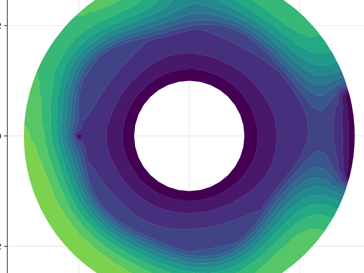

This result is a great match to what we found in the tutorial. If we wanted to convert this mean exit time problem into the corresponding SteadyFVMProblem, we can do:

function T_exact(x, y)
    r = sqrt(x^2 + y^2)
    if r < R₁
        return (R₁^2 - r^2) / (4D₁) + (R₂^2 - R₁^2) / (4D₂)
    else
        return (R₂^2 - r^2) / (4D₂)
    end
end
initial_condition = [T_exact(x, y) for (x, y) in DelaunayTriangulation.each_point(tri)] # an initial guess
fvm_prob = SteadyFVMProblem(FVMProblem(mesh, BCs, ICs;
    diffusion_function=let D = diffusion_function
        (x, y, t, u, p) -> D(x, y, p)
    end,
    diffusion_parameters,
    source_function=(x, y, t, u, p) -> one(u),
    final_time=Inf,
    initial_condition))

SteadyFVMProblem with 1849 nodes

Let's compare the two solutions.

using SteadyStateDiffEq, OrdinaryDiffEq
fvm_sol = solve(fvm_prob, DynamicSS(TRBDF2()))

retcode: Success
u: 1909-element Vector{Float64}:
     0.0
     0.0
     0.0
     0.0
     0.0
     ⋮
 11368.782888840387
  9993.656515673974
 10980.672794386479
 11184.769786986508
  1794.3869214098736

ax = Axis(fig[1, 2], width=600, height=600, title="Template")
tricontourf!(ax, tri, fvm_sol.u, levels=0:1000:15000, extendhigh=:auto)
resize_to_layout!(fig)
fig
ind = findall(i -> DelaunayTriangulation.has_vertex(tri, i), DelaunayTriangulation.each_point_index(tri))

1849-element Vector{Int64}:
    1
    2
    3
    4
    5
    6
    7
    8
    9
   10
    ⋮
 1901
 1902
 1903
 1904
 1905
 1906
 1907
 1908
 1909

Using the Provided Template

Let's now use the built-in MeanExitTimeProblem which implements the above template inside FiniteVolumeMethod.jl.

prob = MeanExitTimeProblem(mesh, BCs, ICs;
    diffusion_function,
    diffusion_parameters)
sol = solve(prob, KLUFactorization())

retcode: Default
u: 1909-element Vector{Float64}:
     0.0
     0.0
     0.0
     0.0
     0.0
     ⋮
 11335.518061726689
  9924.932215598092
 10944.471309084121
 11157.501835643034
  1789.7801237673489

fig, ax, sc = tricontourf(tri, sol.u, levels=0:1000:15000, extendhigh=:auto,
    axis=(width=600, height=600))
fig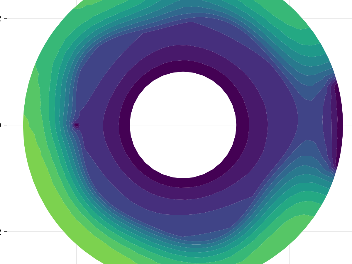

This matches what we have above. To finish, here is a benchmark comparing the approaches.

using BenchmarkTools
@btime solve($prob, $KLUFactorization());

  2.559 ms (56 allocations: 3.72 MiB)

@btime solve($fvm_prob, $DynamicSS($KenCarp47(linsolve=KLUFactorization())));

  221.851 ms (314440 allocations: 90.23 MiB)

Very fast!

Just the code

An uncommented version of this example is given below. You can view the source code for this file here.

function create_met_b!(A, mesh, conditions)
    b = zeros(DelaunayTriangulation.num_points(mesh.triangulation))
    for i in each_solid_vertex(mesh.triangulation)
        if !FVM.is_dirichlet_node(conditions, i)
            b[i] = -1
        else
            A[i, i] = 1.0 # b[i] = is already zero
        end
    end
    return b
end

using FiniteVolumeMethod, SparseArrays, DelaunayTriangulation, LinearSolve
const FVM = FiniteVolumeMethod
function met_problem(mesh::FVMGeometry,
    BCs::BoundaryConditions, # the actual implementation also checks that the types are only Dirichlet/Neumann
    ICs::InternalConditions=InternalConditions();
    diffusion_function,
    diffusion_parameters=nothing)
    conditions = Conditions(mesh, BCs, ICs)
    n = DelaunayTriangulation.num_points(mesh.triangulation)
    A = zeros(n, n)
    FVM.triangle_contributions!(A, mesh, conditions, diffusion_function, diffusion_parameters)
    b = create_met_b!(A, mesh, conditions)
    FVM.fix_missing_vertices!(A, b, mesh)
    return LinearProblem(sparse(A), b)
end

# Define the triangulation
R₁, R₂ = 2.0, 3.0
ε = 0.05
g = θ -> sin(3θ) + cos(5θ)
R1_f = let R₁ = R₁, ε = ε, g = g # use let for type stability
    θ -> R₁ * (1.0 + ε * g(θ))
end
ϵr = 0.25
dirichlet = CircularArc((R₂ * cos(ϵr), R₂ * sin(ϵr)), (R₂ * cos(2π - ϵr), R₂ * sin(2π - ϵr)), (0.0, 0.0))
neumann = CircularArc((R₂ * cos(2π - ϵr), R₂ * sin(2π - ϵr)), (R₂ * cos(ϵr), R₂ * sin(ϵr)), (0.0, 0.0))
hole = CircularArc((0.0, 1.0), (0.0, 1.0), (0.0, 0.0), positive=false)
boundary_nodes = [[[dirichlet], [neumann]], [[hole]]]
points = [(-2.0, 0.0), (0.0, 2.95)]
tri = triangulate(points; boundary_nodes)
θ = LinRange(0, 2π, 250)
xin = @views (@. R1_f(θ) * cos(θ))[begin:end-1]
yin = @views (@. R1_f(θ) * sin(θ))[begin:end-1]
add_point!(tri, xin[1], yin[1])
for i in 2:length(xin)
    add_point!(tri, xin[i], yin[i])
    n = DelaunayTriangulation.num_points(tri)
    add_segment!(tri, n - 1, n)
end
n = DelaunayTriangulation.num_points(tri)
add_segment!(tri, n - 1, n)
pointhole_idxs = [1, 2]
refine!(tri; max_area=1e-3get_area(tri));
# Define the problem
mesh = FVMGeometry(tri)
zero_f = (x, y, t, u, p) -> zero(u) # the function doesn't actually matter, but it still needs to be provided
BCs = BoundaryConditions(mesh, (zero_f, zero_f, zero_f), (Neumann, Dirichlet, Dirichlet))
ICs = InternalConditions((x, y, t, u, p) -> zero(u), dirichlet_nodes=Dict(pointhole_idxs .=> 1))
D₁, D₂ = 6.25e-4, 6.25e-5
diffusion_function = (x, y, p) -> begin
    r = sqrt(x^2 + y^2)
    ϕ = atan(y, x)
    interface_val = p.R1_f(ϕ)
    return r < interface_val ? p.D₁ : p.D₂
end
diffusion_parameters = (D₁=D₁, D₂=D₂, R1_f=R1_f)
prob = met_problem(mesh, BCs, ICs; diffusion_function, diffusion_parameters)

prob.A

sol = solve(prob, KLUFactorization())

using CairoMakie
fig, ax, sc = tricontourf(tri, sol.u, levels=0:1000:15000, extendhigh=:auto,
    axis=(width=600, height=600, title="Template"))
fig

function T_exact(x, y)
    r = sqrt(x^2 + y^2)
    if r < R₁
        return (R₁^2 - r^2) / (4D₁) + (R₂^2 - R₁^2) / (4D₂)
    else
        return (R₂^2 - r^2) / (4D₂)
    end
end
initial_condition = [T_exact(x, y) for (x, y) in DelaunayTriangulation.each_point(tri)] # an initial guess
fvm_prob = SteadyFVMProblem(FVMProblem(mesh, BCs, ICs;
    diffusion_function=let D = diffusion_function
        (x, y, t, u, p) -> D(x, y, p)
    end,
    diffusion_parameters,
    source_function=(x, y, t, u, p) -> one(u),
    final_time=Inf,
    initial_condition))

using SteadyStateDiffEq, OrdinaryDiffEq
fvm_sol = solve(fvm_prob, DynamicSS(TRBDF2()))

ax = Axis(fig[1, 2], width=600, height=600, title="Template")
tricontourf!(ax, tri, fvm_sol.u, levels=0:1000:15000, extendhigh=:auto)
resize_to_layout!(fig)
fig
ind = findall(i -> DelaunayTriangulation.has_vertex(tri, i), DelaunayTriangulation.each_point_index(tri))

prob = MeanExitTimeProblem(mesh, BCs, ICs;
    diffusion_function,
    diffusion_parameters)
sol = solve(prob, KLUFactorization())

fig, ax, sc = tricontourf(tri, sol.u, levels=0:1000:15000, extendhigh=:auto,
    axis=(width=600, height=600))
fig

This page was generated using Literate.jl.