Diffusion Equation on an Annulus

In this tutorial, we consider a diffusion equation on an annulus:

\[\begin{equation} \begin{aligned} \pdv{u(\vb x, t)}{t} &= \grad^2 u(\vb x, t) & \vb x \in \Omega, \\ \grad u(\vb x, t) \vdot \vu n(\vb x) &= 0 & \vb x \in \mathcal D(0, 1), \\ u(\vb x, t) &= c(t) & \vb x \in \mathcal D(0,0.2), \\ u(\vb x, t) &= u_0(\vb x), \end{aligned} \end{equation}\]

demonstrating how we can solve PDEs over multiply-connected domains. Here, $\mathcal D(0, r)$ is a circle of radius $r$ centred at the origin, $\Omega$ is the annulus between $\mathcal D(0,0.2)$ and $\mathcal D(0, 1)$, $c(t) = 50[1-\mathrm{e}^{-t/2}]$, and

\[u_0(x) = 10\mathrm{e}^{-25\left[\left(x+\frac12\right)^2+\left(y+\frac12\right)^2\right]} - 10\mathrm{e}^{-45\left[\left(x-\frac12\right)^2+\left(y-\frac12\right)^2\right]} - 5\mathrm{e}^{-50\left[\left(x+\frac{3}{10}\right)^2+\left(y+\frac12\right)^2\right]}.\]

For the mesh, we use two CircularArcs to define the annulus.

using DelaunayTriangulation, FiniteVolumeMethod, CairoMakie
R₁, R₂ = 0.2, 1.0
inner = CircularArc((R₁, 0.0), (R₁, 0.0), (0.0, 0.0), positive=false)
outer = CircularArc((R₂, 0.0), (R₂, 0.0), (0.0, 0.0))
boundary_nodes = [[[outer]], [[inner]]]
points = NTuple{2,Float64}[]
tri = triangulate(points; boundary_nodes)
A = get_area(tri)
refine!(tri; max_area=1e-4A)
triplot(tri)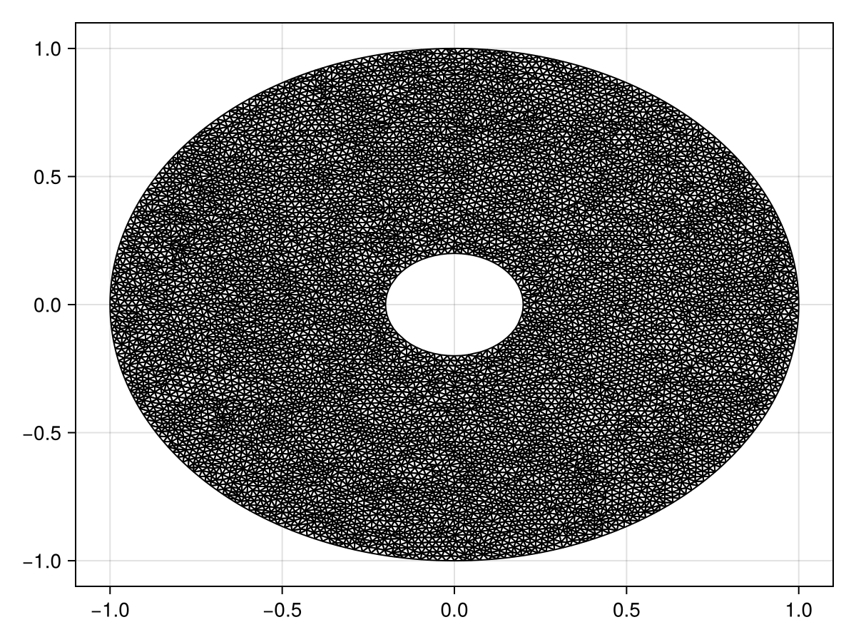

mesh = FVMGeometry(tri)

FVMGeometry with 8986 control volumes, 17657 triangles, and 26643 edges

Now let us define the boundary conditions. Remember, the order of the boundary conditions follows the order of the boundaries in the mesh. The outer boundary came first, and then came the inner boundary. We can verify that this is the order of the boundary indices as follows:

fig = Figure()
ax = Axis(fig[1, 1])
outer = [get_point(tri, i) for i in get_neighbours(tri, -1)]
inner = [get_point(tri, i) for i in get_neighbours(tri, -2)]
triplot!(ax, tri)
scatter!(ax, outer, color=:red)
scatter!(ax, inner, color=:blue)
fig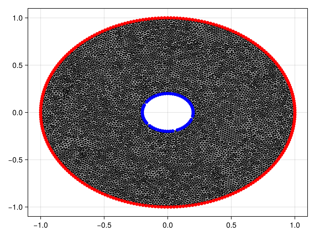

So, the boundary conditions are:

outer_bc = (x, y, t, u, p) -> zero(u)
inner_bc = (x, y, t, u, p) -> oftype(u, 50(1 - exp(-t / 2)))
types = (Neumann, Dirichlet)
BCs = BoundaryConditions(mesh, (outer_bc, inner_bc), types)

BoundaryConditions with 2 boundary conditions with types (Neumann, Dirichlet)

Finally, let's define the problem and solve it.

initial_condition_f = (x, y) -> begin
    10 * exp(-25 * ((x + 0.5) * (x + 0.5) + (y + 0.5) * (y + 0.5))) - 5 * exp(-50 * ((x + 0.3) * (x + 0.3) + (y + 0.5) * (y + 0.5))) - 10 * exp(-45 * ((x - 0.5) * (x - 0.5) + (y - 0.5) * (y - 0.5)))
end
diffusion_function = (x, y, t, u, p) -> one(u)
initial_condition = [initial_condition_f(x, y) for (x, y) in DelaunayTriangulation.each_point(tri)]
final_time = 2.0
prob = FVMProblem(mesh, BCs;
    diffusion_function,
    final_time,
    initial_condition)

FVMProblem with 8986 nodes and time span (0.0, 2.0)

using OrdinaryDiffEq, LinearSolve
sol = solve(prob, TRBDF2(linsolve=KLUFactorization()), saveat=0.2)

retcode: Success
Interpolation: 1st order linear
t: 11-element Vector{Float64}:
 0.0
 0.2
 0.4
 0.6
 0.8
 1.0
 1.2
 1.4
 1.6
 1.8
 2.0
u: 11-element Vector{Vector{Float64}}:
 [-1.6918979226151304e-9, -2.1738750708653327e-6, 3.726653172035993e-5, -1.6918979226151364e-9, 3.705953483484758e-5, -0.2105979106615764, 5.175555005801385e-16, 1.1709299175694265, 5.1755544523350865e-16, 0.0020233820430370225  …  1.017027715370349e-12, -4.2235113212980827e-7, -3.304946603943528e-13, -0.004551592181902057, -0.0064304765914936154, 8.721736999482021e-13, -1.1528805500311166, 8.447171031958781, 2.978359285676185e-11, 1.0817587716627684e-11]
 [0.04117910195045892, 4.673029309079141, 0.8990653696612744, 0.05110297689026207, 0.8306226003678054, -0.16747201171959292, 0.4445510417191181, 1.147051624751615, 0.4029356709116486, 4.673029309079141  …  0.4909240565115158, 12.90636806408303, 0.5584901470451944, 0.22509408820619672, 0.20290115293711325, 0.4772265653493249, 0.023392929726039565, 1.2302871430206754, 0.5764339052043608, 0.5583052682723283]
 [1.84290422245115, 8.312130701094134, 2.2505959472306527, 1.8537690436184904, 2.2311692298644266, 1.7700052057623754, 2.049893555918292, 2.329223609084653, 2.0292946146849378, 8.312130701094134  …  2.224918563863111, 21.720032765875807, 2.484595384773257, 2.2625806765973833, 2.2331352755669496, 2.176304728887901, 2.0411303593179744, 2.5875702814010078, 2.1980307171508815, 2.1592307263759087]
 [4.361848033234305, 12.865947654000854, 4.544890624171355, 4.367406857228138, 4.538309775710649, 4.32878170847978, 4.456257442160016, 4.579114439145473, 4.448267353197731, 12.865947654000854  …  4.706394293876565, 32.95941957200919, 5.0749273820291885, 4.899953039009057, 4.865599513119467, 4.637015007438031, 4.653592067030615, 4.9285106440055655, 4.613630957703188, 4.562784833967426]
 [7.258725147070201, 15.398463716249378, 7.339648317111258, 7.2607239416463365, 7.337779371562839, 7.243612699799387, 7.300019516333157, 7.355276325643119, 7.297932349327238, 15.398463716249378  …  7.586814389715068, 25.811670003251844, 8.008180432989844, 7.854303811150692, 7.817457983898861, 7.507298711420576, 7.595075248343087, 7.748793393066147, 7.462923869118641, 7.406155405195243]
 [10.313140415756969, 19.416305213947815, 10.347976026660668, 10.313334376655472, 10.348091749481613, 10.306192306162178, 10.330174089767418, 10.35535544659824, 10.3307842866666, 19.416305213947815  …  10.628540943520438, 81.32412451673143, 11.064939996087158, 10.923505102147004, 10.88629445077354, 10.545907517731804, 10.663552864436992, 10.761725096362726, 10.493010252955, 10.434543331513408]
 [13.378623116782679, 22.165008972225763, 13.392700164361301, 13.377979903803045, 13.39367773063749, 13.37536468044711, 13.384701877479607, 13.396372999879716, 13.38650542722287, 22.165008972225763  …  13.680967973882263, 106.05436784800668, 14.113379574857118, 13.980717434727321, 13.94423988827793, 13.598968626878497, 13.72669846348104, 13.798556017728929, 13.543621910392536, 13.485820608738658]
 [16.359835773706397, 24.945358456714583, 16.364626141117117, 16.358835348794376, 16.365954346276794, 16.35824125404706, 16.361039215393202, 16.366618580449483, 16.363317937957028, 24.945358456714583  …  16.646446897211113, 97.26615003032128, 17.06227195248694, 16.937929082847877, 16.903021043965534, 16.567497655598114, 16.695143650049967, 16.75341798091734, 16.51295639161479, 16.457385575192212]
 [19.201516466400637, 26.33191680589102, 19.202207120685433, 19.200389551053416, 19.203646718059034, 19.20067584673791, 19.200605480976584, 19.203425847607644, 19.203019982842186, 26.33191680589102  …  19.471984141214033, 35.560360227350515, 19.868339201997376, 19.751053595286187, 19.71783256419596, 19.396877277239124, 19.520394119253684, 19.57107760812444, 19.344456900610172, 19.291677879145038]
 [21.872821495511094, 29.051659422966658, 21.871769157259443, 21.871680478949735, 21.87320331725962, 21.872324916032696, 21.871059944064864, 21.87261878537958, 21.87344006066417, 29.051659422966658  …  22.123918347248267, 128.98319315418533, 22.491997405333343, 22.383838918090568, 22.35303544308569, 22.054002610490546, 22.169834120767486, 22.21489208229165, 22.004917307080508, 21.955759370944453]
 [24.361300531757756, 30.390275045183962, 24.359559123866017, 24.36019643750569, 24.360936741007734, 24.36096666345112, 24.359249144580318, 24.360222624146363, 24.361525863922132, 30.390275045183962  …  24.595475594301856, 30.078225101256542, 24.93975768558161, 24.838805349169093, 24.809999723966047, 24.53013845745168, 24.63879433985803, 24.679983425444778, 24.484164662961497, 24.4382545638098]

fig = Figure(fontsize=38)
for (i, j) in zip(1:3, (1, 6, 11))
    local ax
    ax = Axis(fig[1, i], width=600, height=600,
        xlabel="x", ylabel="y",
        title="t = $(sol.t[j])",
        titlealign=:left)
    tricontourf!(ax, tri, sol.u[j], levels=-10:2:40, colormap=:matter)
    tightlimits!(ax)
end
resize_to_layout!(fig)
fig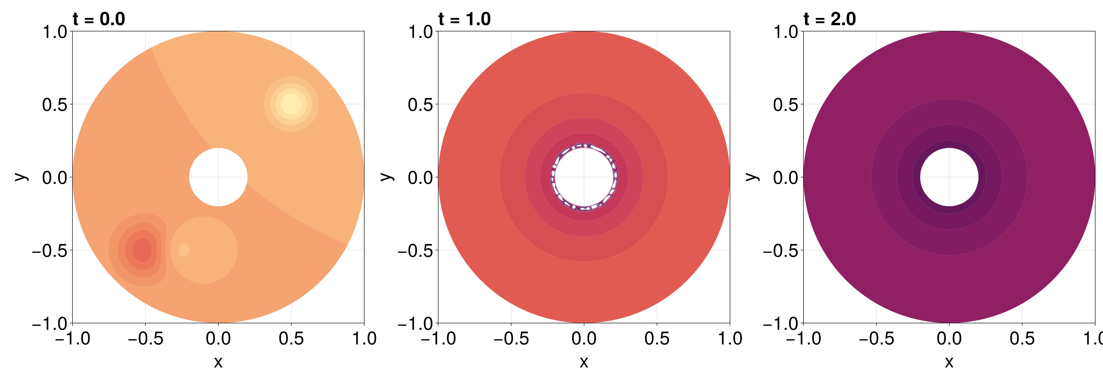

To finish this example, let us consider how natural neighbour interpolation can be applied here. The application is more complicated for this problem since the mesh has holes. Before we do that, though, let us show how we could use pl_interpolate, which could be useful if we did not need a higher quality interpolant. Let us interpolate the solution at $t = 1$, which is sol.t[6]. For this, we need to put the ghost triangles back into tri so that we can safely apply jump_and_march. This is done with add_ghost_triangles!.

add_ghost_triangles!(tri)

Delaunay Triangulation.
   Number of vertices: 8986
   Number of triangles: 17657
   Number of edges: 26643
   Has boundary nodes: true
   Has ghost triangles: true
   Curve-bounded: true
   Weighted: false
   Constrained: true

(Actually, tri already had these ghost triangles, but we are just showing how you would add them back in if needed.)

Now let's interpolate.

x = LinRange(-R₂, R₂, 400)
y = LinRange(-R₂, R₂, 400)
interp_vals = zeros(length(x), length(y))
u = sol.u[6]
last_triangle = Ref((1, 1, 1))
for (j, _y) in enumerate(y)
    for (i, _x) in enumerate(x)
        T = jump_and_march(tri, (_x, _y), try_points=last_triangle[])
        last_triangle[] = triangle_vertices(T) # used to accelerate jump_and_march, since the points we're looking for are close to each other
        if DelaunayTriangulation.is_ghost_triangle(T) # don't extrapolate
            interp_vals[i, j] = NaN
        else
            interp_vals[i, j] = pl_interpolate(prob, T, sol.u[6], _x, _y)
        end
    end
end
fig, ax, sc = contourf(x, y, interp_vals, levels=-10:2:40, colormap=:matter)
fig

Let's now consider applying NaturalNeighbours.jl. We apply it naively first to highlight some complications.

using NaturalNeighbours
_x = vec([x for x in x, y in y]) # NaturalNeighbours.jl needs vector data
_y = vec([y for x in x, y in y])
itp = interpolate(tri, u, derivatives=true)

Natural Neighbour Interpolant
    z: [10.313140415756969, 19.416305213947815, 10.347976026660668, 10.313334376655472, 10.348091749481613, 10.306192306162178, 10.330174089767418, 10.35535544659824, 10.3307842866666, 19.416305213947815  …  10.628540943520438, 81.32412451673143, 11.064939996087158, 10.923505102147004, 10.88629445077354, 10.545907517731804, 10.663552864436992, 10.761725096362726, 10.493010252955, 10.434543331513408]
    ∇: [(-0.007043658467826603, -0.015804756791782417), (8069.183360228173, 348.3680031688037), (0.017930354356131575, -0.022260476280995884), (-0.028536368978853394, -0.018854937606489694), (-0.015351704720132864, 0.006094591652674357), (-0.0037368562078451692, 0.002020063111958764), (0.026913666035249712, -0.059162740653517606), (-0.0066350989770403105, -0.002502801489900407), (-0.020565808276781405, -0.018480604332588066), (-8142.970804595418, 80.25782541097756)  …  (-2.4100526654101753, 2.1895314454909918), (9.988489429753864, -648.2328100490213), (2.4014669609515416, -4.8430257716605105), (-0.9940755063805305, -4.755842530047819), (-1.0417431007914824, -4.568076125891664), (-1.9518658157237296, 1.9116378451889298), (-1.780987307583375, -3.1179184039275087), (2.8392070207364544, 2.595195196258463), (1.8461079740976578, -1.4020267335003636), (1.4444321902807433, -1.0968767778658686)]
    H: [(14.87975185062579, 0.06639634089831305, 0.11616618527644132), (-751649.6319676217, 43861.99146277773, 9382.94211384727), (14.394048125738793, 0.14325842659101967, -0.08225272984822053), (0.09649523705338404, 13.679393673014058, -0.20944776943134358), (0.06026548318686057, 14.449028635164089, 0.001966355253401152), (7.2698487245563035, 7.477299598899117, 7.446038948694327), (6.1345054990320325, 6.147005968634387, -5.68064298070243), (8.058925055238237, 8.016196734679852, 7.93636625991287), (7.307714731016173, 7.551825013212107, -7.537449248839009), (-776616.5917949318, 39397.89098382128, 16291.026157237588)  …  (8.33972714706266, 6.679989232691314, -11.492466823057757), (-13978.641153632441, -325031.2184457859, 61948.03937050247), (-1.6918249852031693, 16.41509715518848, -12.145012115706903), (-5.448266585046659, 20.79583265918094, 5.686893483219091), (-5.12882204343735, 20.25096986137513, 5.98698837501413), (7.709343349380333, 7.461771373570749, -10.88315961919536), (1.2892118630472438, 13.721283405989423, 10.402129492521881), (8.658536281594223, 6.272209451437896, 12.455563172139136), (10.71199404141495, 4.686693260784345, -9.866318196967311), (10.391893948645833, 4.617566175336629, -9.283413016938814)]

itp_vals = itp(_x, _y; method=Farin())

160000-element Vector{Float64}:
 10.355341754004353
 10.355351418278211
 10.355361082552067
 10.355370746825924
 10.35538041109978
  ⋮
 10.306252720547526
 10.306229332891899
 10.306205945236272
 10.306182557580646
 10.30615916992502

fig, ax, sc = contourf(x, y, reshape(itp_vals, length(x), length(y)), colormap=:matter, levels=-10:2:40)
fig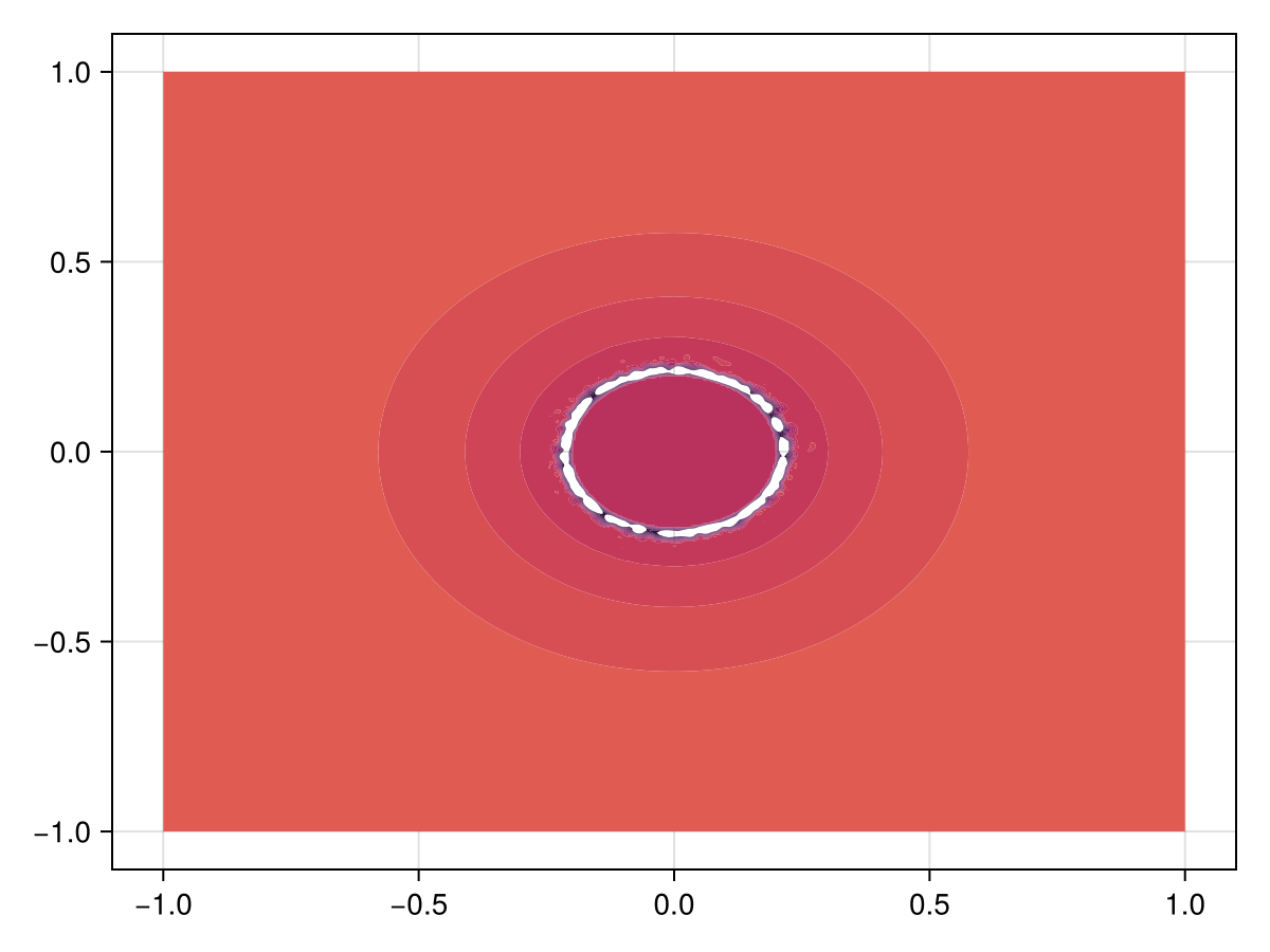

The issue here is that the interpolant is trying to extrapolate inside the hole and outside of the annulus. To avoid this, you need to pass project=false.

itp_vals = itp(_x, _y; method=Farin(), project=false)

160000-element Vector{Float64}:
 Inf
 Inf
 Inf
 Inf
 Inf
  ⋮
 Inf
 Inf
 Inf
 Inf
 Inf

fig, ax, sc = contourf(x, y, reshape(itp_vals, length(x), length(y)), colormap=:matter, levels=-10:2:40)
fig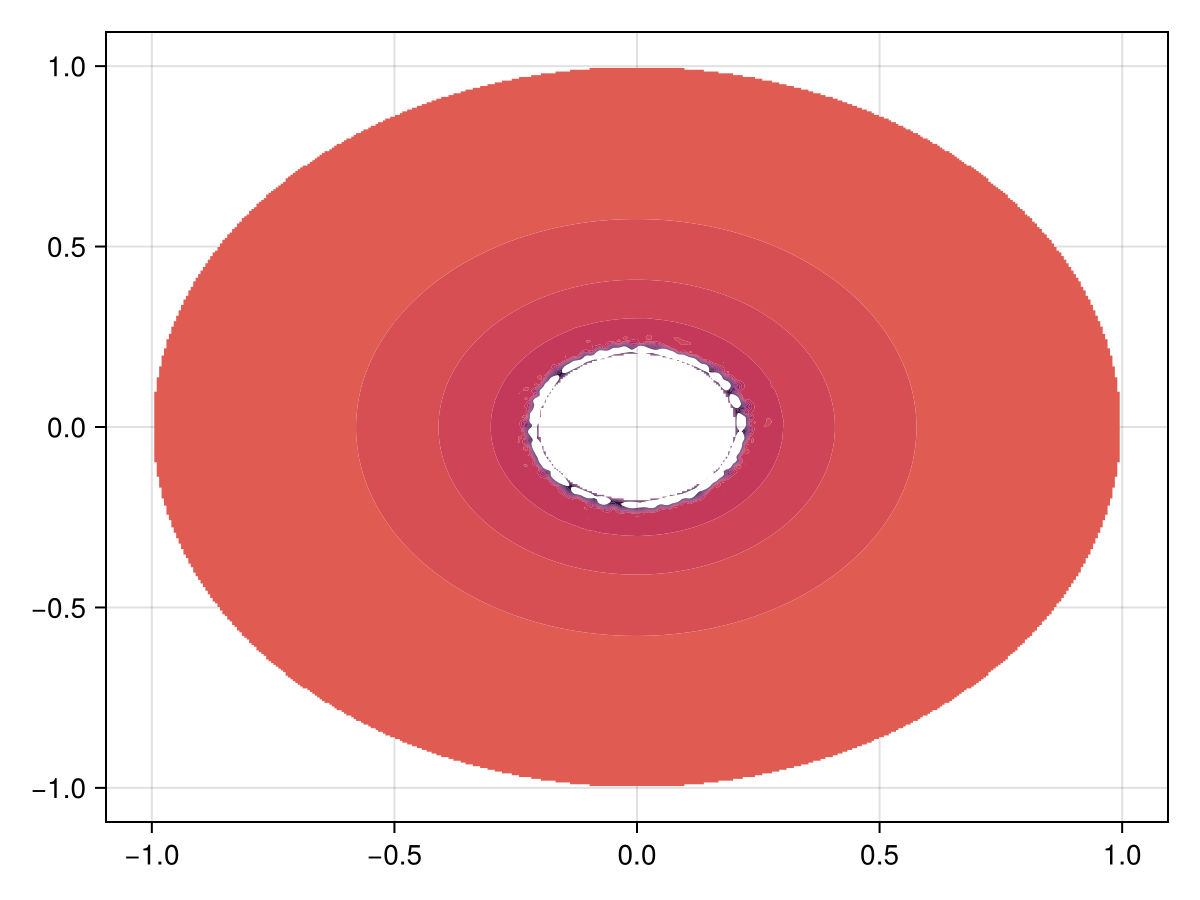

Just the code

An uncommented version of this example is given below. You can view the source code for this file here.

using DelaunayTriangulation, FiniteVolumeMethod, CairoMakie
R₁, R₂ = 0.2, 1.0
inner = CircularArc((R₁, 0.0), (R₁, 0.0), (0.0, 0.0), positive=false)
outer = CircularArc((R₂, 0.0), (R₂, 0.0), (0.0, 0.0))
boundary_nodes = [[[outer]], [[inner]]]
points = NTuple{2,Float64}[]
tri = triangulate(points; boundary_nodes)
A = get_area(tri)
refine!(tri; max_area=1e-4A)
triplot(tri)

mesh = FVMGeometry(tri)

fig = Figure()
ax = Axis(fig[1, 1])
outer = [get_point(tri, i) for i in get_neighbours(tri, -1)]
inner = [get_point(tri, i) for i in get_neighbours(tri, -2)]
triplot!(ax, tri)
scatter!(ax, outer, color=:red)
scatter!(ax, inner, color=:blue)
fig

outer_bc = (x, y, t, u, p) -> zero(u)
inner_bc = (x, y, t, u, p) -> oftype(u, 50(1 - exp(-t / 2)))
types = (Neumann, Dirichlet)
BCs = BoundaryConditions(mesh, (outer_bc, inner_bc), types)

initial_condition_f = (x, y) -> begin
    10 * exp(-25 * ((x + 0.5) * (x + 0.5) + (y + 0.5) * (y + 0.5))) - 5 * exp(-50 * ((x + 0.3) * (x + 0.3) + (y + 0.5) * (y + 0.5))) - 10 * exp(-45 * ((x - 0.5) * (x - 0.5) + (y - 0.5) * (y - 0.5)))
end
diffusion_function = (x, y, t, u, p) -> one(u)
initial_condition = [initial_condition_f(x, y) for (x, y) in DelaunayTriangulation.each_point(tri)]
final_time = 2.0
prob = FVMProblem(mesh, BCs;
    diffusion_function,
    final_time,
    initial_condition)

using OrdinaryDiffEq, LinearSolve
sol = solve(prob, TRBDF2(linsolve=KLUFactorization()), saveat=0.2)

fig = Figure(fontsize=38)
for (i, j) in zip(1:3, (1, 6, 11))
    local ax
    ax = Axis(fig[1, i], width=600, height=600,
        xlabel="x", ylabel="y",
        title="t = $(sol.t[j])",
        titlealign=:left)
    tricontourf!(ax, tri, sol.u[j], levels=-10:2:40, colormap=:matter)
    tightlimits!(ax)
end
resize_to_layout!(fig)
fig

add_ghost_triangles!(tri)

x = LinRange(-R₂, R₂, 400)
y = LinRange(-R₂, R₂, 400)
interp_vals = zeros(length(x), length(y))
u = sol.u[6]
last_triangle = Ref((1, 1, 1))
for (j, _y) in enumerate(y)
    for (i, _x) in enumerate(x)
        T = jump_and_march(tri, (_x, _y), try_points=last_triangle[])
        last_triangle[] = triangle_vertices(T) # used to accelerate jump_and_march, since the points we're looking for are close to each other
        if DelaunayTriangulation.is_ghost_triangle(T) # don't extrapolate
            interp_vals[i, j] = NaN
        else
            interp_vals[i, j] = pl_interpolate(prob, T, sol.u[6], _x, _y)
        end
    end
end
fig, ax, sc = contourf(x, y, interp_vals, levels=-10:2:40, colormap=:matter)
fig

using NaturalNeighbours
_x = vec([x for x in x, y in y]) # NaturalNeighbours.jl needs vector data
_y = vec([y for x in x, y in y])
itp = interpolate(tri, u, derivatives=true)

itp_vals = itp(_x, _y; method=Farin())

fig, ax, sc = contourf(x, y, reshape(itp_vals, length(x), length(y)), colormap=:matter, levels=-10:2:40)
fig

itp_vals = itp(_x, _y; method=Farin(), project=false)

fig, ax, sc = contourf(x, y, reshape(itp_vals, length(x), length(y)), colormap=:matter, levels=-10:2:40)
fig

This page was generated using Literate.jl.