Poisson's Equation

Poisson's Equation

We now write a solver for Poisson's equation. What we produce in this section can also be accessed in FiniteVolumeMethod.PoissonsEquation.

Mathematical Details

We start by describing the mathematical details. The problems we will be solving take the form

\[\div[D(\vb x)\grad u] = f(\vb x).\]

Note that this is very similar to a mean exit time problem, except $f(\vb x) = -1$ for mean exit time problems. Note that this is actually a generalised Poisson equation - typically these equations look like $\grad^2 u = f$.^[1]

From these similarities, we already know that

\[\frac{1}{V_i}\sum_{\sigma\in\mathcal E_i} D(\vb x_\sigma)\left[\left(s_{k, 11}n_\sigma^x+s_{k,21}n_\sigma^y\right)u_{k1} + \left(s_{k,12}n_\sigma^x+s_{k,22}n_\sigma^y\right)u_{k2}+\left(s_{k,13}n_\sigma^x+s_{k,23}n_\sigma^y\right)u_{k3}\right]L_\sigma = f(\vb x_i),\]

and thus we can write this as $\vb a_i^{\mkern-1.5mu\mathsf T}\vb u = b_i$ as usual, with $b_i = f(\vb x_i)$. The boundary conditions are handled in the same way as in mean exit time problems.

Implementation

Let us now implement our problem. For mean exit time problems, we had a function create_met_b that we used for defining $\vb b$. We should generalise that function to now accept a source function:

function create_rhs_b(mesh, conditions, source_function, source_parameters)
    b = zeros(DelaunayTriangulation.num_points(mesh.triangulation))
    for i in each_solid_vertex(mesh.triangulation)
        if !FVM.is_dirichlet_node(conditions, i)
            p = get_point(mesh, i)
            x, y = getxy(p)
            b[i] = source_function(x, y, source_parameters)
        end
    end
    return b
end

create_rhs_b (generic function with 1 method)

We also need a function that applies the Dirichlet conditions.

function apply_steady_dirichlet_conditions!(A, b, mesh, conditions)
    for (i, function_index) in FVM.get_dirichlet_nodes(conditions)
        x, y = get_point(mesh, i)
        b[i] = FVM.eval_condition_fnc(conditions, function_index, x, y, nothing, nothing)
        A[i, i] = 1.0
    end
end

apply_steady_dirichlet_conditions! (generic function with 1 method)

So, our problem can be defined by:

using FiniteVolumeMethod, SparseArrays, DelaunayTriangulation, LinearSolve
const FVM = FiniteVolumeMethod
function poissons_equation(mesh::FVMGeometry,
    BCs::BoundaryConditions,
    ICs::InternalConditions=InternalConditions();
    diffusion_function=(x,y,p)->1.0,
    diffusion_parameters=nothing,
    source_function,
    source_parameters=nothing)
    conditions = Conditions(mesh, BCs, ICs)
    n = DelaunayTriangulation.num_points(mesh.triangulation)
    A = zeros(n, n)
    b = create_rhs_b(mesh, conditions, source_function, source_parameters)
    FVM.triangle_contributions!(A, mesh, conditions, diffusion_function, diffusion_parameters)
    FVM.boundary_edge_contributions!(A, b, mesh, conditions, diffusion_function, diffusion_parameters)
    apply_steady_dirichlet_conditions!(A, b, mesh, conditions)
    FVM.fix_missing_vertices!(A, b, mesh)
    return LinearProblem(sparse(A), b)
end

poissons_equation (generic function with 2 methods)

Now let's test this problem. We consider

\[\begin{equation*} \begin{aligned} \grad^2 u &= -\sin(\pi x)\sin(\pi y) & \vb x \in [0,1]^2, \\ u &= 0 & \vb x \in\partial[0,1]^2. \end{aligned} \end{equation*}\]

tri = triangulate_rectangle(0, 1, 0, 1, 100, 100, single_boundary=true)
mesh = FVMGeometry(tri)
BCs = BoundaryConditions(mesh, (x, y, t, u, p) -> zero(x), Dirichlet)
source_function = (x, y, p) -> -sin(π * x) * sin(π * y)
prob = poissons_equation(mesh, BCs;  source_function)

LinearProblem. In-place: true
b: 10000-element Vector{Float64}:
 0.0
 0.0
 0.0
 0.0
 0.0
 ⋮
 0.0
 0.0
 0.0
 0.0
 0.0

sol = solve(prob, KLUFactorization())

retcode: Default
u: 10000-element Vector{Float64}:
 0.0
 0.0
 0.0
 0.0
 0.0
 ⋮
 0.0
 0.0
 0.0
 0.0
 0.0

using CairoMakie
fig, ax, sc = tricontourf(tri, sol.u, levels=LinRange(0, 0.05, 10), colormap=:matter, extendhigh=:auto)
tightlimits!(ax)
fig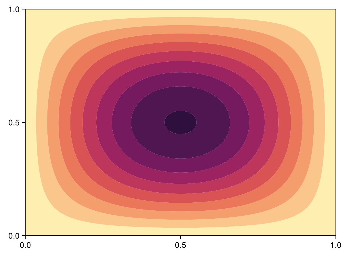

If we wanted to turn this into a SteadyFVMProblem, we use a similar call to poissons_equation above except with an initial_condition for the initial guess. Moreover, we need to change the sign of the source function, since above we are solving $\div[D(\vb x)\grad u] = f(\vb x)$, when FVMProblems assume that we are solving $0 = \div[D(\vb x)\grad u] + f(\vb x)$.

initial_condition = zeros(DelaunayTriangulation.num_points(tri))
fvm_prob = SteadyFVMProblem(FVMProblem(mesh, BCs;
    diffusion_function= (x, y, t, u, p) -> 1.0,
    source_function=let S = source_function
        (x, y, t, u, p) -> -S(x, y, p)
    end,
    initial_condition,
    final_time=Inf))

SteadyFVMProblem with 10000 nodes

using SteadyStateDiffEq, OrdinaryDiffEq
fvm_sol = solve(fvm_prob, DynamicSS(TRBDF2(linsolve=KLUFactorization())))

retcode: Success
u: 10000-element Vector{Float64}:
 0.0
 0.0
 0.0
 0.0
 0.0
 ⋮
 0.0
 0.0
 0.0
 0.0
 0.0

Using the Provided Template

Let's now use the built-in PoissonsEquation which implements the above template inside FiniteVolumeMethod.jl. The above problem can be constructed as follows:

prob = PoissonsEquation(mesh, BCs; source_function=source_function)

PoissonsEquation with 10000 nodes

sol = solve(prob, KLUFactorization())

retcode: Default
u: 10000-element Vector{Float64}:
 0.0
 0.0
 0.0
 0.0
 0.0
 ⋮
 0.0
 0.0
 0.0
 0.0
 0.0

Here is a benchmark comparison of the PoissonsEquation approach against the FVMProblem approach.

using BenchmarkTools
@btime solve($prob, $KLUFactorization());

  15.442 ms (56 allocations: 15.21 MiB)

@btime solve($fvm_prob, $DynamicSS(TRBDF2(linsolve=KLUFactorization())));

  189.406 ms (185761 allocations: 93.63 MiB)

Let's now also solve a generalised Poisson equation. Based on Section 7 of this paper by Nagel (2012), we consider an equation of the form

\[\div\left[\epsilon(\vb x)\grad V(\vb x)\right] = -\frac{\rho(\vb x)}{\epsilon_0}.\]

We consider this equation on the domain $\Omega = [0, 10]^2$. We put two parallel capacitor plates inside the domain, with the first in $2 \leq x \leq 8$ along $y = 3$, and the other at $2 \leq x \leq 8$ along $y=7$. We use $V = 1$ on the top plate, and $V = -1$ on the bottom plate. For the domain boundaries, $\partial\Omega$, we use homogeneous Dirichlet conditions on the top and bottom sides, and homogeneous Neumann conditions on the left and right sides. For the space-varying electric constant $\epsilon(\vb x)$, we use^[2]

\[\epsilon(\vb x) = 1 + \frac12(\epsilon_0 - 1)\left[1 + \erf\left(\frac{r}{\Delta}\right)\right],\]

where $r$ is the distance between $\vb x$ and the parallel plates, $\Delta = 4$. The value of $\epsilon_0$ is approximately $\epsilon_0 = 8.8541878128 \times 10^{-12}$. For the charge density $\rho(\vb x)$, we use a Gaussian density,

\[\rho(\vb x) = \frac{Q}{2\pi}\mathrm{e}^{-r^2/2},\]

where, again, $r$ is the distance between $\vb x$ and the parallel plates, and $Q = 10^{-6}$.

To define this problem, let us first define the mesh. We will need to manually put in the capacitor plates so that we can enforce Dirichlet conditions on them.

a, b, c, d = 0.0, 10.0, 0.0, 10.0
e, f = (2.0, 3.0), (8.0, 3.0)
g, h = (2.0, 7.0), (8.0, 7.0)
points = [(a, c), (b, c), (b, d), (a, d), e, f, g, h]
boundary_nodes = [[1, 2], [2, 3], [3, 4], [4, 1]]
segments = Set(((5, 6), (7, 8)))
tri = triangulate(points; boundary_nodes, segments, delete_ghosts=false)
refine!(tri; max_area=1e-4get_area(tri))
fig, ax, sc = triplot(tri, show_constrained_edges=true, constrained_edge_linewidth=5)
fig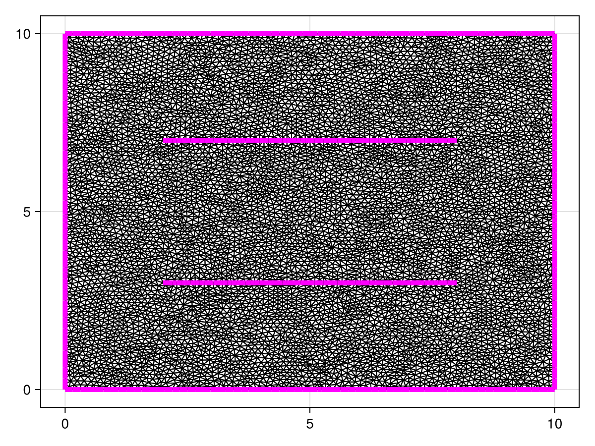

mesh = FVMGeometry(tri)

FVMGeometry with 8067 control volumes, 15861 triangles, and 23927 edges

The boundary conditions are given by:

zero_f = (x, y, t, u, p) -> zero(x)
bc_f = (zero_f, zero_f, zero_f, zero_f)
bc_types = (Dirichlet, Neumann, Dirichlet, Neumann) # bot, right, top, left
BCs = BoundaryConditions(mesh, bc_f, bc_types)

BoundaryConditions with 4 boundary conditions with types (Dirichlet, Neumann, Dirichlet, Neumann)

To define the internal conditions, we need to get the indices for the plates.

function find_vertices_on_plates(tri)
    lower_plate = Int[]
    upper_plate = Int[]
    for i in each_solid_vertex(tri)
        x, y = get_point(tri, i)
        in_range = 2 ≤ x ≤ 8
        if in_range
            y == 3 && push!(lower_plate, i)
            y == 7 && push!(upper_plate, i)
        end
    end
    return lower_plate, upper_plate
end
lower_plate, upper_plate = find_vertices_on_plates(tri)
dirichlet_nodes = Dict(
    (lower_plate .=> 1)...,
    (upper_plate .=> 2)...
)
internal_f = ((x, y, t, u, p) -> -one(x), (x, y, t, u, p) -> one(x))
ICs = InternalConditions(internal_f, dirichlet_nodes=dirichlet_nodes)

InternalConditions with 114 Dirichlet nodes and 0 Dudt nodes

Next, we define $\epsilon(\vb x)$ and $\rho(\vb x)$. We need a function that computes the distance between a point and the plates. For the distance between a point and a line segment, we can use:^[3]

using LinearAlgebra
function dist_to_line(p, a, b)
    ℓ² = norm(a .- b)^2
    t = max(0.0, min(1.0, dot(p .- a, b .- a) / ℓ²))
    pv = a .+ t .* (b .- a)
    return norm(p .- pv)
end

dist_to_line (generic function with 1 method)

Thus, the distance between a point and the two plates is:

function dist_to_plates(x, y)
    p = (x, y)
    a1, b1 = (2.0, 3.0), (8.0, 3.0)
    a2, b2 = (2.0, 7.0), (8.0, 7.0)
    d1 = dist_to_line(p, a1, b1)
    d2 = dist_to_line(p, a2, b2)
    return min(d1, d2)
end

dist_to_plates (generic function with 1 method)

So, our function $\epsilon(\vb x)$ is defined by:

using SpecialFunctions
function dielectric_function(x, y, p)
    r = dist_to_plates(x, y)
    return 1 + (p.ϵ₀ - 1) * (1 + erf(r / p.Δ)) / 2
end

dielectric_function (generic function with 1 method)

The charge density is:

function charge_density(x, y, p)
    r = dist_to_plates(x, y)
    return p.Q / (2π) * exp(-r^2 / 2)
end

charge_density (generic function with 1 method)

Using this charge density, our source function is defined by:

function plate_source_function(x, y, p)
    ρ = charge_density(x, y, p)
    return -ρ / p.ϵ₀
end

plate_source_function (generic function with 1 method)

Now we can define our problem.

diffusion_parameters = (ϵ₀=8.8541878128e-12, Δ=4.0)
source_parameters = (ϵ₀=8.8541878128e-12, Q=1e-6)
prob = PoissonsEquation(mesh, BCs, ICs;
    diffusion_function=dielectric_function,
    diffusion_parameters=diffusion_parameters,
    source_function=plate_source_function,
    source_parameters=source_parameters)

PoissonsEquation with 8067 nodes

sol = solve(prob, KLUFactorization())

retcode: Default
u: 8236-element Vector{Float64}:
     0.0
     0.0
     0.0
     0.0
    -1.0
     ⋮
 51581.29690932709
 47170.6367481186
 19483.0891565168
 10348.595996812204
 25143.353653799924

With this solution, we can also define the electric field $\vb E$, using $\vb E = -\grad V$. To compute the gradients, we use NaturalNeighbours.jl.

using NaturalNeighbours
itp = interpolate(tri, sol.u; derivatives=true)
E = map(.-, itp.gradient) # E = -∇V

8236-element Vector{Tuple{Float64, Float64}}:
 (75.13669911167318, -38842.702565145155)
 (-111.13250797982077, -38903.32630425008)
 (-114.87720892138049, 39038.059776912174)
 (185.9037051987188, 38914.27359862993)
 (69026.16186674804, -12174.554406884647)
 ⋮
 (-11838.032704900921, -10193.190254302626)
 (-7991.769258646464, 6192.032617852947)
 (2696.069948845957, -22493.037752129632)
 (-4.5677003197312755, 42087.29626954362)
 (-2208.181073809621, -8959.118222759382)

For plotting the electric field, we will show the electric field intensity $\|\vb E\|$, and we can also show the arrows. Rather than showing all arrows, we will show them at a smaller grid of values, which requires differentiating itp so that we can get the gradients at arbitary points.

∂ = differentiate(itp, 1)
x = LinRange(0, 10, 25)
y = LinRange(0, 10, 25)
x_vec = [x for x in x, y in y] |> vec
y_vec = [y for x in x, y in y] |> vec
E_itp = map(.-, ∂(x_vec, y_vec, interpolant_method=Hiyoshi(2)))
E_intensity = norm.(E_itp)
fig = Figure(fontsize=38)
ax = Axis(fig[1, 1], width=600, height=600, titlealign=:left,
    xlabel="x", ylabel="y", title="Voltage")
tricontourf!(ax, tri, sol.u, levels=15, colormap=:ocean)
arrow_positions = [Point2f(x, y) for (x, y) in zip(x_vec, y_vec)]
arrow_directions = [Point2f(e...) for e in E_itp]
arrows!(ax, arrow_positions, arrow_directions,
    lengthscale=0.3, normalize=true, arrowcolor=E_intensity, linecolor=E_intensity)
    xlims!(ax,0,10)
    ylims!(ax,0,10)
ax = Axis(fig[1, 2], width=600, height=600, titlealign=:left,
    xlabel="x", ylabel="y", title="Electric Field")
tricontourf!(ax, tri, norm.(E), levels=15, colormap=:ocean)
arrows!(ax, arrow_positions, arrow_directions,
    lengthscale=0.3, normalize=true, arrowcolor=E_intensity, linecolor=E_intensity)
xlims!(ax,0,10)
ylims!(ax,0,10)
resize_to_layout!(fig)
fig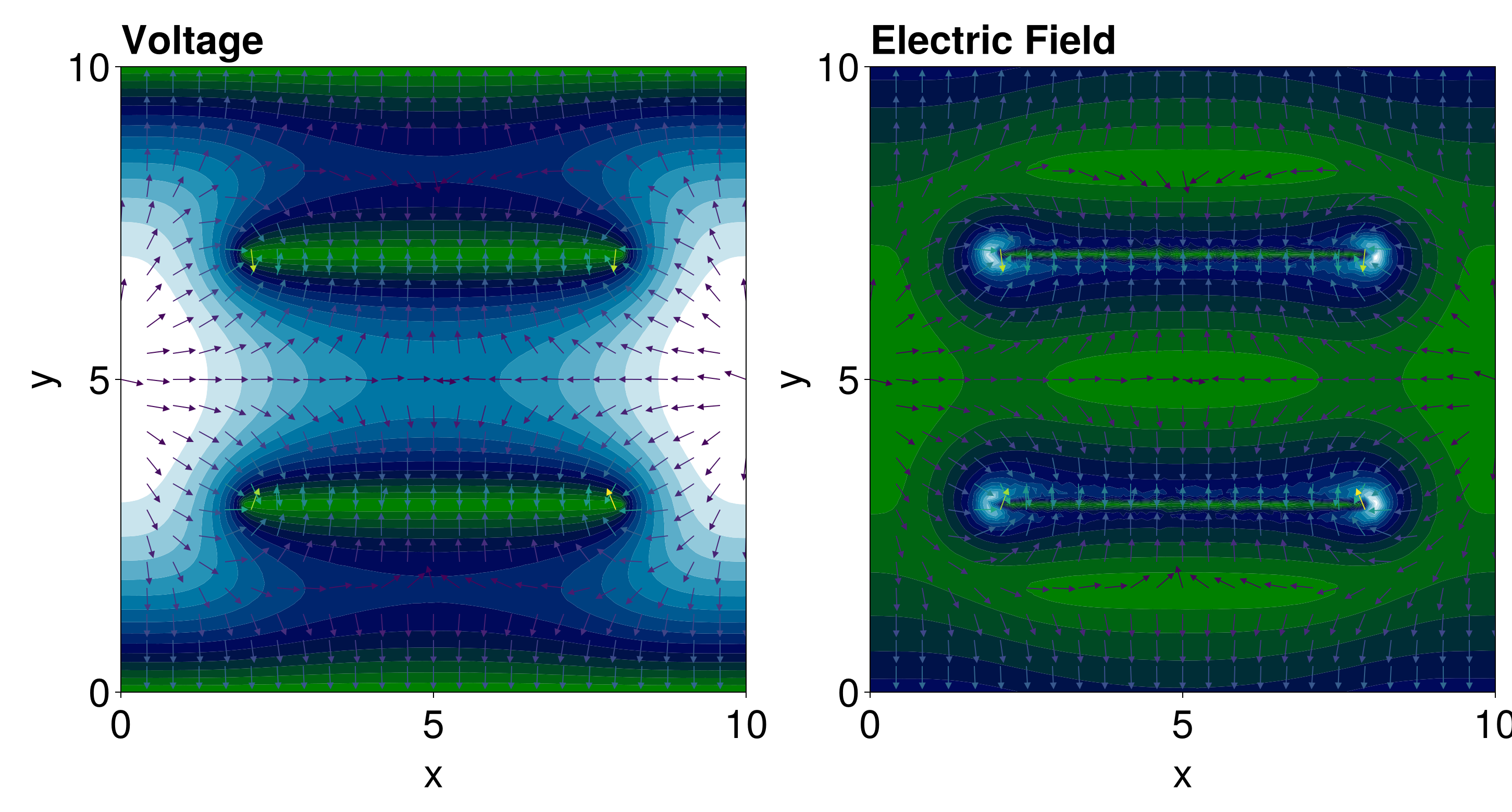

To finish, let us benchmark the PoissonsEquation approach against the FVMProblem approach.

fvm_prob = SteadyFVMProblem(FVMProblem(mesh, BCs, ICs;
    diffusion_function=let D = dielectric_function
        (x, y, t, u, p) -> D(x, y, p)
    end,
    source_function=let S = plate_source_function
        (x, y, t, u, p) -> -S(x, y, p)
    end,
    diffusion_parameters=diffusion_parameters,
    source_parameters=source_parameters,
    initial_condition=zeros(DelaunayTriangulation.num_points(tri)),
    final_time=Inf))

SteadyFVMProblem with 8067 nodes

@btime solve($prob, $KLUFactorization());

  9.061 ms (56 allocations: 10.81 MiB)

@btime solve($fvm_prob, $DynamicSS(TRBDF2(linsolve=KLUFactorization())));

  329.327 ms (201134 allocations: 93.70 MiB)

Just the code

An uncommented version of this example is given below. You can view the source code for this file here.

function create_rhs_b(mesh, conditions, source_function, source_parameters)
    b = zeros(DelaunayTriangulation.num_points(mesh.triangulation))
    for i in each_solid_vertex(mesh.triangulation)
        if !FVM.is_dirichlet_node(conditions, i)
            p = get_point(mesh, i)
            x, y = getxy(p)
            b[i] = source_function(x, y, source_parameters)
        end
    end
    return b
end

function apply_steady_dirichlet_conditions!(A, b, mesh, conditions)
    for (i, function_index) in FVM.get_dirichlet_nodes(conditions)
        x, y = get_point(mesh, i)
        b[i] = FVM.eval_condition_fnc(conditions, function_index, x, y, nothing, nothing)
        A[i, i] = 1.0
    end
end

using FiniteVolumeMethod, SparseArrays, DelaunayTriangulation, LinearSolve
const FVM = FiniteVolumeMethod
function poissons_equation(mesh::FVMGeometry,
    BCs::BoundaryConditions,
    ICs::InternalConditions=InternalConditions();
    diffusion_function=(x,y,p)->1.0,
    diffusion_parameters=nothing,
    source_function,
    source_parameters=nothing)
    conditions = Conditions(mesh, BCs, ICs)
    n = DelaunayTriangulation.num_points(mesh.triangulation)
    A = zeros(n, n)
    b = create_rhs_b(mesh, conditions, source_function, source_parameters)
    FVM.triangle_contributions!(A, mesh, conditions, diffusion_function, diffusion_parameters)
    FVM.boundary_edge_contributions!(A, b, mesh, conditions, diffusion_function, diffusion_parameters)
    apply_steady_dirichlet_conditions!(A, b, mesh, conditions)
    FVM.fix_missing_vertices!(A, b, mesh)
    return LinearProblem(sparse(A), b)
end

tri = triangulate_rectangle(0, 1, 0, 1, 100, 100, single_boundary=true)
mesh = FVMGeometry(tri)
BCs = BoundaryConditions(mesh, (x, y, t, u, p) -> zero(x), Dirichlet)
source_function = (x, y, p) -> -sin(π * x) * sin(π * y)
prob = poissons_equation(mesh, BCs;  source_function)

sol = solve(prob, KLUFactorization())

using CairoMakie
fig, ax, sc = tricontourf(tri, sol.u, levels=LinRange(0, 0.05, 10), colormap=:matter, extendhigh=:auto)
tightlimits!(ax)
fig

initial_condition = zeros(DelaunayTriangulation.num_points(tri))
fvm_prob = SteadyFVMProblem(FVMProblem(mesh, BCs;
    diffusion_function= (x, y, t, u, p) -> 1.0,
    source_function=let S = source_function
        (x, y, t, u, p) -> -S(x, y, p)
    end,
    initial_condition,
    final_time=Inf))

using SteadyStateDiffEq, OrdinaryDiffEq
fvm_sol = solve(fvm_prob, DynamicSS(TRBDF2(linsolve=KLUFactorization())))

prob = PoissonsEquation(mesh, BCs; source_function=source_function)

sol = solve(prob, KLUFactorization())

a, b, c, d = 0.0, 10.0, 0.0, 10.0
e, f = (2.0, 3.0), (8.0, 3.0)
g, h = (2.0, 7.0), (8.0, 7.0)
points = [(a, c), (b, c), (b, d), (a, d), e, f, g, h]
boundary_nodes = [[1, 2], [2, 3], [3, 4], [4, 1]]
segments = Set(((5, 6), (7, 8)))
tri = triangulate(points; boundary_nodes, segments, delete_ghosts=false)
refine!(tri; max_area=1e-4get_area(tri))
fig, ax, sc = triplot(tri, show_constrained_edges=true, constrained_edge_linewidth=5)
fig

mesh = FVMGeometry(tri)

zero_f = (x, y, t, u, p) -> zero(x)
bc_f = (zero_f, zero_f, zero_f, zero_f)
bc_types = (Dirichlet, Neumann, Dirichlet, Neumann) # bot, right, top, left
BCs = BoundaryConditions(mesh, bc_f, bc_types)

function find_vertices_on_plates(tri)
    lower_plate = Int[]
    upper_plate = Int[]
    for i in each_solid_vertex(tri)
        x, y = get_point(tri, i)
        in_range = 2 ≤ x ≤ 8
        if in_range
            y == 3 && push!(lower_plate, i)
            y == 7 && push!(upper_plate, i)
        end
    end
    return lower_plate, upper_plate
end
lower_plate, upper_plate = find_vertices_on_plates(tri)
dirichlet_nodes = Dict(
    (lower_plate .=> 1)...,
    (upper_plate .=> 2)...
)
internal_f = ((x, y, t, u, p) -> -one(x), (x, y, t, u, p) -> one(x))
ICs = InternalConditions(internal_f, dirichlet_nodes=dirichlet_nodes)

using LinearAlgebra
function dist_to_line(p, a, b)
    ℓ² = norm(a .- b)^2
    t = max(0.0, min(1.0, dot(p .- a, b .- a) / ℓ²))
    pv = a .+ t .* (b .- a)
    return norm(p .- pv)
end

function dist_to_plates(x, y)
    p = (x, y)
    a1, b1 = (2.0, 3.0), (8.0, 3.0)
    a2, b2 = (2.0, 7.0), (8.0, 7.0)
    d1 = dist_to_line(p, a1, b1)
    d2 = dist_to_line(p, a2, b2)
    return min(d1, d2)
end

using SpecialFunctions
function dielectric_function(x, y, p)
    r = dist_to_plates(x, y)
    return 1 + (p.ϵ₀ - 1) * (1 + erf(r / p.Δ)) / 2
end

function charge_density(x, y, p)
    r = dist_to_plates(x, y)
    return p.Q / (2π) * exp(-r^2 / 2)
end

function plate_source_function(x, y, p)
    ρ = charge_density(x, y, p)
    return -ρ / p.ϵ₀
end

diffusion_parameters = (ϵ₀=8.8541878128e-12, Δ=4.0)
source_parameters = (ϵ₀=8.8541878128e-12, Q=1e-6)
prob = PoissonsEquation(mesh, BCs, ICs;
    diffusion_function=dielectric_function,
    diffusion_parameters=diffusion_parameters,
    source_function=plate_source_function,
    source_parameters=source_parameters)

sol = solve(prob, KLUFactorization())

using NaturalNeighbours
itp = interpolate(tri, sol.u; derivatives=true)
E = map(.-, itp.gradient) # E = -∇V

∂ = differentiate(itp, 1)
x = LinRange(0, 10, 25)
y = LinRange(0, 10, 25)
x_vec = [x for x in x, y in y] |> vec
y_vec = [y for x in x, y in y] |> vec
E_itp = map(.-, ∂(x_vec, y_vec, interpolant_method=Hiyoshi(2)))
E_intensity = norm.(E_itp)
fig = Figure(fontsize=38)
ax = Axis(fig[1, 1], width=600, height=600, titlealign=:left,
    xlabel="x", ylabel="y", title="Voltage")
tricontourf!(ax, tri, sol.u, levels=15, colormap=:ocean)
arrow_positions = [Point2f(x, y) for (x, y) in zip(x_vec, y_vec)]
arrow_directions = [Point2f(e...) for e in E_itp]
arrows!(ax, arrow_positions, arrow_directions,
    lengthscale=0.3, normalize=true, arrowcolor=E_intensity, linecolor=E_intensity)
    xlims!(ax,0,10)
    ylims!(ax,0,10)
ax = Axis(fig[1, 2], width=600, height=600, titlealign=:left,
    xlabel="x", ylabel="y", title="Electric Field")
tricontourf!(ax, tri, norm.(E), levels=15, colormap=:ocean)
arrows!(ax, arrow_positions, arrow_directions,
    lengthscale=0.3, normalize=true, arrowcolor=E_intensity, linecolor=E_intensity)
xlims!(ax,0,10)
ylims!(ax,0,10)
resize_to_layout!(fig)
fig

fvm_prob = SteadyFVMProblem(FVMProblem(mesh, BCs, ICs;
    diffusion_function=let D = dielectric_function
        (x, y, t, u, p) -> D(x, y, p)
    end,
    source_function=let S = plate_source_function
        (x, y, t, u, p) -> -S(x, y, p)
    end,
    diffusion_parameters=diffusion_parameters,
    source_parameters=source_parameters,
    initial_condition=zeros(DelaunayTriangulation.num_points(tri)),
    final_time=Inf))

This page was generated using Literate.jl.

1See, for example, this paper.
2This form of $\epsilon(\vb x)$ is based on this paper by Fisicaro et al. (2016).
3Taken from here.