Equilibrium Temperature Distribution with Mixed Boundary Conditions and using EnsembleProblems

For this tutorial, we consider the following problem:

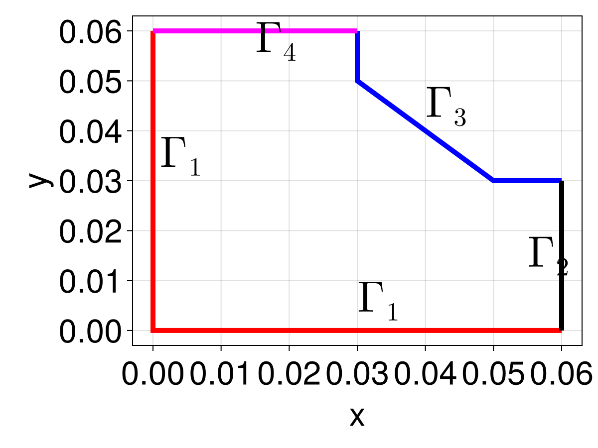
\[\begin{equation} \begin{aligned} \grad^2 T &= 0 & \vb x \in \Omega, \\ \grad T \vdot \vu n &= 0 & \vb x \in \Gamma_1, \\ T &= 40 & \vb x \in \Gamma_2, \\ k\grad T \vdot \vu n &= h(T_{\infty} - T) & \vb x \in \Gamma_3, \\ T &= 70 & \vb x \in \Gamma_4. \\ \end{aligned} \end{equation}\]

This domain $\Omega$ with boundary $\partial\Omega=\Gamma_1\cup\Gamma_2\cup\Gamma_3\cup\Gamma_4$ is shown below.

Let us start by defining the mesh.

using DelaunayTriangulation, FiniteVolumeMethod, CairoMakie
A, B, C, D, E, F, G = (0.0, 0.0),
(0.06, 0.0),
(0.06, 0.03),
(0.05, 0.03),
(0.03, 0.05),
(0.03, 0.06),
(0.0, 0.06)
bn1 = [G, A, B]
bn2 = [B, C]
bn3 = [C, D, E, F]
bn4 = [F, G]
bn = [bn1, bn2, bn3, bn4]
boundary_nodes, points = convert_boundary_points_to_indices(bn)
tri = triangulate(points; boundary_nodes)
refine!(tri; max_area=1e-4get_area(tri))
triplot(tri)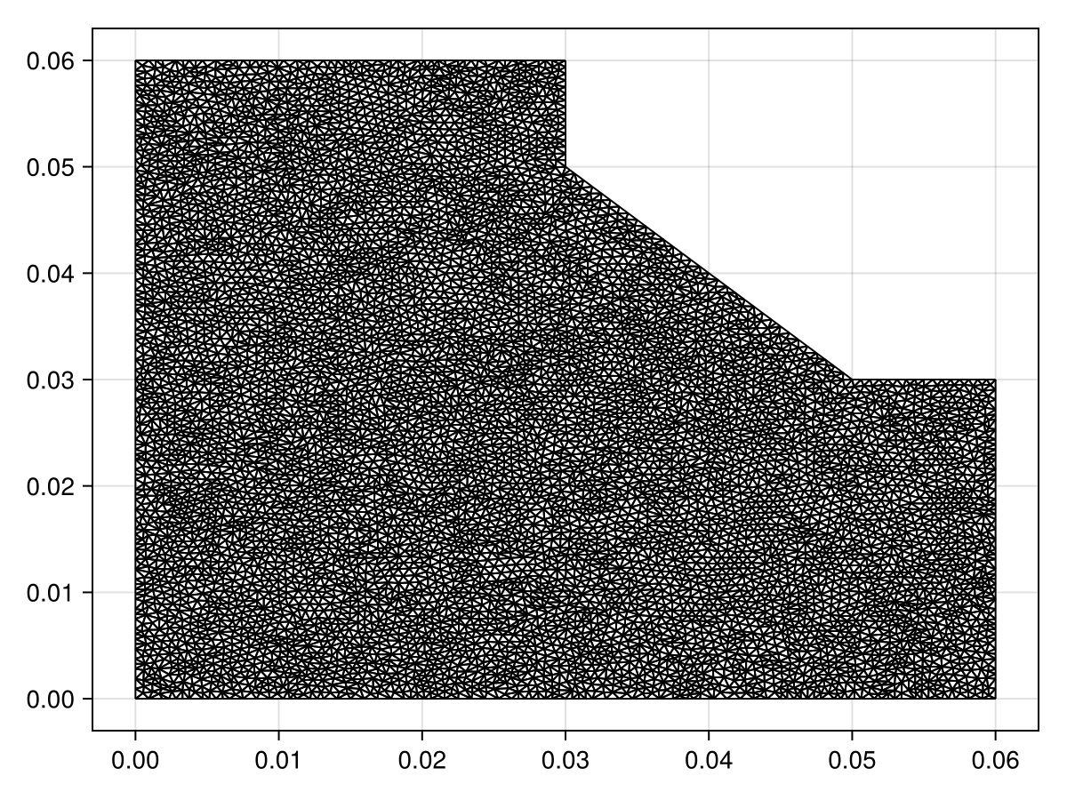

mesh = FVMGeometry(tri)

FVMGeometry with 8144 control volumes, 15944 triangles, and 24087 edges

For the boundary conditions, the parameters that we use are $k = 3$, $h = 20$, and $T_{\infty} = 20$ for thermal conductivity, heat transfer coefficient, and ambient temperature, respectively.

k = 3.0
h = 20.0
T∞ = 20.0
bc1 = (x, y, t, T, p) -> zero(T) # ∇T⋅n=0
bc2 = (x, y, t, T, p) -> oftype(T, 40.0) # T=40
bc3 = (x, y, t, T, p) -> -p.h * (p.T∞- T) / p.k # k∇T⋅n=h(T∞-T). The minus is since q = -∇T
bc4 = (x, y, t, T, p) -> oftype(T, 70.0) # T=70
parameters = (nothing, nothing, (h=h, T∞=T∞, k=k), nothing)
BCs = BoundaryConditions(mesh, (bc1, bc2, bc3, bc4),
    (Neumann, Dirichlet, Neumann, Dirichlet);
    parameters)

BoundaryConditions with 4 boundary conditions with types (Neumann, Dirichlet, Neumann, Dirichlet)

Now we can define the actual problem. For the initial condition, which recall is used as an initial guess for steady state problems, let us use an initial condition which ranges from $T=70$ at $y=0.06$ down to $T=40$ at $y=0$.

diffusion_function = (x, y, t, T, p) -> one(T)
f = (x, y) -> 500y + 40
initial_condition = [f(x, y) for (x, y) in DelaunayTriangulation.each_point(tri)]
final_time = Inf
prob = FVMProblem(mesh, BCs;
    diffusion_function,
    initial_condition,
    final_time)

FVMProblem with 8144 nodes and time span (0.0, Inf)

steady_prob = SteadyFVMProblem(prob)

SteadyFVMProblem with 8144 nodes

Now we can solve.

using OrdinaryDiffEq, SteadyStateDiffEq
sol = solve(steady_prob, DynamicSS(Rosenbrock23()))

retcode: Success
u: 8277-element Vector{Float64}:
 70.0
 53.103092183130336
 40.0
 40.0
 44.13431924538936
  ⋮
 54.71768793632413
 53.77066316067286
 53.221394119351224
 49.03373489007241
 49.984596496529385

fig, ax, sc = tricontourf(tri, sol.u, levels=40:70, axis=(xlabel="x", ylabel="y"))
fig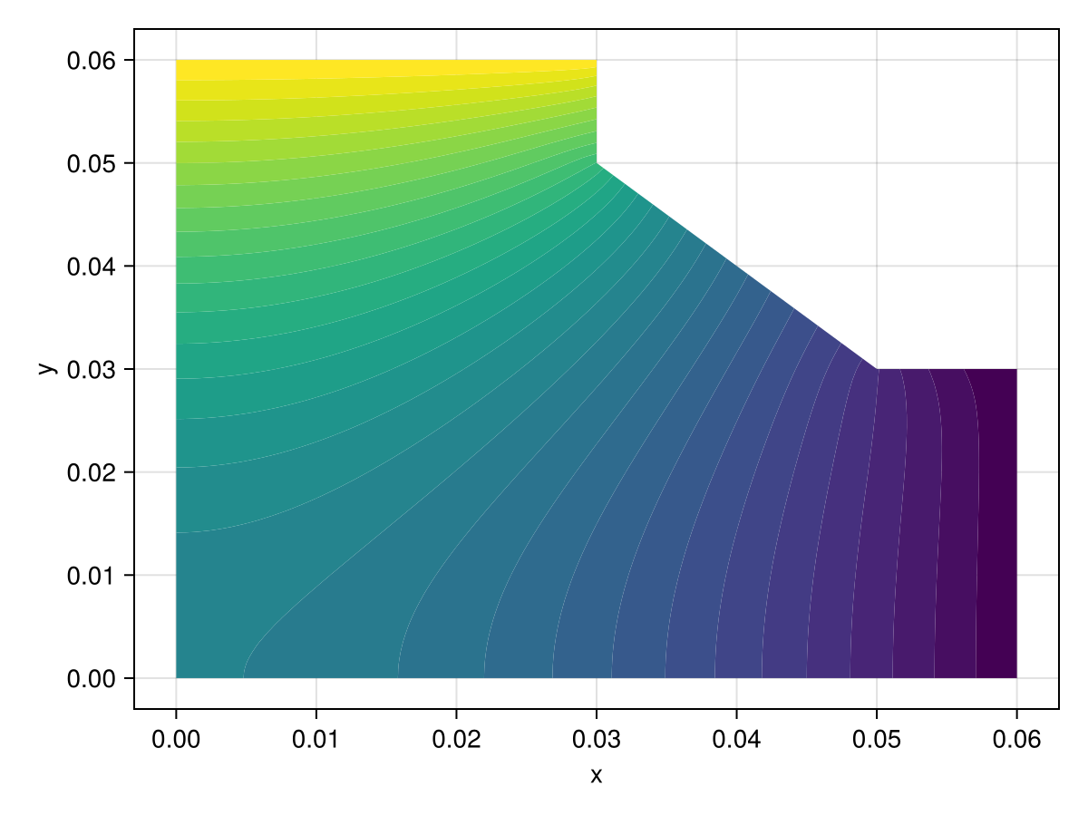

Just the code

An uncommented version of this example is given below. You can view the source code for this file here.

using DelaunayTriangulation, FiniteVolumeMethod, CairoMakie
A, B, C, D, E, F, G = (0.0, 0.0),
(0.06, 0.0),
(0.06, 0.03),
(0.05, 0.03),
(0.03, 0.05),
(0.03, 0.06),
(0.0, 0.06)
bn1 = [G, A, B]
bn2 = [B, C]
bn3 = [C, D, E, F]
bn4 = [F, G]
bn = [bn1, bn2, bn3, bn4]
boundary_nodes, points = convert_boundary_points_to_indices(bn)
tri = triangulate(points; boundary_nodes)
refine!(tri; max_area=1e-4get_area(tri))
triplot(tri)

mesh = FVMGeometry(tri)

k = 3.0
h = 20.0
T∞ = 20.0
bc1 = (x, y, t, T, p) -> zero(T) # ∇T⋅n=0
bc2 = (x, y, t, T, p) -> oftype(T, 40.0) # T=40
bc3 = (x, y, t, T, p) -> -p.h * (p.T∞- T) / p.k # k∇T⋅n=h(T∞-T). The minus is since q = -∇T
bc4 = (x, y, t, T, p) -> oftype(T, 70.0) # T=70
parameters = (nothing, nothing, (h=h, T∞=T∞, k=k), nothing)
BCs = BoundaryConditions(mesh, (bc1, bc2, bc3, bc4),
    (Neumann, Dirichlet, Neumann, Dirichlet);
    parameters)

diffusion_function = (x, y, t, T, p) -> one(T)
f = (x, y) -> 500y + 40
initial_condition = [f(x, y) for (x, y) in DelaunayTriangulation.each_point(tri)]
final_time = Inf
prob = FVMProblem(mesh, BCs;
    diffusion_function,
    initial_condition,
    final_time)

steady_prob = SteadyFVMProblem(prob)

using OrdinaryDiffEq, SteadyStateDiffEq
sol = solve(steady_prob, DynamicSS(Rosenbrock23()))

fig, ax, sc = tricontourf(tri, sol.u, levels=40:70, axis=(xlabel="x", ylabel="y"))
fig

This page was generated using Literate.jl.