Linear Reaction-Diffusion Equations

• Linear Reaction-Diffusion Equations
• • Mathematical Details
  • Implementation
  • Using the Provided Template
  • Just the code

Next, we write a specialised solver for solving linear reaction-diffusion equations. What we produce in this section can also be accessed in FiniteVolumeMethod.LinearReactionDiffusionEquation.

Mathematical Details

To start, let's give the mathematical details. The problems we will be solving take the form

\[\pdv{u}{t} = \div\left[D(\vb x)\grad u\right] + f(\vb x)u.\]

We want to turn this into an equation of the form $\mathrm d\vb u/\mathrm dt = \vb A\vb u + \vb b$ as usual. This takes the same form as our diffusion equation example, except with the extra $f(\vb x)u$ term, which just adds an exta $f(\vb x)$ term to the diagonal of $\vb A$. See the previois sections for further mathematical details.

Implementation

Let us now implement the solver. For constructing $\vb A$, we can use FiniteVolumeMethod.triangle_contributions! as in the previous sections, but we will need an extra function to add $f(\vb x)$ to the appropriate diagonals. We can also reuse apply_dirichlet_conditions!, apply_dudt_conditions, and boundary_edge_contributions! from the diffusion equation example. Here is our implementation.

using FiniteVolumeMethod, SparseArrays, OrdinaryDiffEq, LinearAlgebra
const FVM = FiniteVolumeMethod
function linear_source_contributions!(A, mesh, conditions, source_function, source_parameters)
    for i in each_solid_vertex(mesh.triangulation)
        if !FVM.has_condition(conditions, i)
            x, y = get_point(mesh, i)
            A[i, i] += source_function(x, y, source_parameters)
        end
    end
end
function linear_reaction_diffusion_equation(mesh::FVMGeometry,
    BCs::BoundaryConditions,
    ICs::InternalConditions=InternalConditions();
    diffusion_function,
    diffusion_parameters=nothing,
    source_function,
    source_parameters=nothing,
    initial_condition,
    initial_time=0.0,
    final_time)
    conditions = Conditions(mesh, BCs, ICs)
    n = DelaunayTriangulation.num_solid_vertices(mesh.triangulation)
    Afull = zeros(n + 1, n + 1)
    A = @views Afull[begin:end-1, begin:end-1]
    b = @views Afull[begin:end-1, end]
    _ic = vcat(initial_condition, 1)
    FVM.triangle_contributions!(A, mesh, conditions, diffusion_function, diffusion_parameters)
    FVM.boundary_edge_contributions!(A, b, mesh, conditions, diffusion_function, diffusion_parameters)
    linear_source_contributions!(A, mesh, conditions, source_function, source_parameters)
    FVM.apply_dudt_conditions!(b, mesh, conditions)
    FVM.apply_dirichlet_conditions!(_ic, mesh, conditions)
    FVM.fix_missing_vertices!(A, b, mesh)
    Af = sparse(Afull)
    prob = ODEProblem(MatrixOperator(Af), _ic, (initial_time, final_time))
    return prob
end

linear_reaction_diffusion_equation (generic function with 2 methods)

If you go and look back at the diffusion_equation function from the diffusion equation example, you will see that this is essentially the same function except we now have linear_source_contributions! and source_function and source_parameters arguments.

Let's now test this function. We consider the problem

\[\pdv{T}{t} = \div\left[10^{-3}x^2y\grad T\right] + (x-1)(y-1)T, \quad \vb x \in [0,1]^2,\]

with $\grad T \vdot\vu n = 1$ on the boundary.

using DelaunayTriangulation
tri = triangulate_rectangle(0, 1, 0, 1, 150, 150, single_boundary=true)
mesh = FVMGeometry(tri)
BCs = BoundaryConditions(mesh, (x, y, t, u, p) -> one(x), Neumann)
diffusion_function = (x, y, p) -> p.D * x^2 * y
diffusion_parameters = (D=1e-3,)
source_function = (x, y, p) -> (x - 1) * (y - 1)
initial_condition = [x^2 + y^2 for (x, y) in DelaunayTriangulation.each_point(tri)]
final_time = 8.0
prob = linear_reaction_diffusion_equation(mesh, BCs;
    diffusion_function, diffusion_parameters,
    source_function, initial_condition, final_time)

ODEProblem with uType Vector{Float64} and tType Float64. In-place: true
timespan: (0.0, 8.0)
u0: 22501-element Vector{Float64}:
 0.0
 4.504301608035674e-5
 0.00018017206432142696
 0.00040538714472321063
 0.0007206882572857079
 ⋮
 1.9601369307688843
 1.9733345344804287
 1.986622224224134
 2.0
 1.0

sol = solve(prob, Tsit5(); saveat=2)

retcode: Success
Interpolation: 1st order linear
t: 5-element Vector{Float64}:
 0.0
 2.0
 4.0
 6.0
 8.0
u: 5-element Vector{Vector{Float64}}:
 [0.0, 4.504301608035674e-5, 0.00018017206432142696, 0.00040538714472321063, 0.0007206882572857079, 0.0011260754020089186, 0.0016215485788928425, 0.0022071077879374803, 0.0028827530291428314, 0.0036484843025088956  …  1.8955002026935723, 1.9082473762443133, 1.921084635827215, 1.9340119814422772, 1.9470294130895003, 1.9601369307688843, 1.9733345344804287, 1.986622224224134, 2.0, 1.0]
 [5.392972715241145e-10, 0.00032839693136766827, 0.001296075999065779, 0.0028772909445736244, 0.005046982038098887, 0.007780761845897446, 0.011054900287088444, 0.014846309987847448, 0.019132531927487154, 0.023891721371031467  …  1.8576012589945818, 1.8669187520665425, 1.8756974896729597, 1.8847638872813472, 1.8917905883397685, 1.9028816744450412, 1.9023588060998364, 1.9299909590795588, 1.8825038119829294, 1.0]
 [7.916735417539239e-9, 0.0023942552773780707, 0.009323370071034585, 0.020421920082540596, 0.03534389913584282, 0.05376187635010668, 0.07536617230272617, 0.09986406790939091, 0.12697904481386757, 0.1564500561223996  …  1.8509136105141937, 1.8585916000411657, 1.866489590050211, 1.873127279309115, 1.8825835388683478, 1.8841164955936183, 1.9053114182151547, 1.876217336879789, 1.9784909725172137, 1.0]
 [8.716291359760385e-8, 0.017455872288248374, 0.0670679181630475, 0.14494671157302416, 0.24751160642335776, 0.3714705521119457, 0.5138009456452595, 0.6717316202228371, 0.8427259076096082, 1.0244657148949745  …  1.8560527056511602, 1.8629729344954407, 1.8696298850566524, 1.8768276955243501, 1.882405374461048, 1.8921110913752748, 1.8912408526896256, 1.9171352722223847, 1.872868756743993, 1.0]
 [8.530436664276848e-7, 0.1272660020066089, 0.4824543028839772, 1.0287720968254568, 1.733305483676693, 2.5666820729791855, 3.5027585194801247, 4.518332688313118, 5.592878646428218, 6.708302802132737  …  1.870052628640883, 1.8761847240549532, 1.8825065061307933, 1.8884430772243854, 1.8956204922796471, 1.8997921608963413, 1.9118930576758824, 1.9042189244693284, 1.9487417968531984, 1.0]

using CairoMakie
fig = Figure(fontsize=38)
for j in eachindex(sol)
    ax = Axis(fig[1, j], width=600, height=600,
        xlabel="x", ylabel="y",
        title="t = $(sol.t[j])")
    tricontourf!(ax, tri, sol.u[j], levels=0:0.1:1, extendlow=:auto, extendhigh=:auto, colormap=:turbo)
    tightlimits!(ax)
end
resize_to_layout!(fig)
fig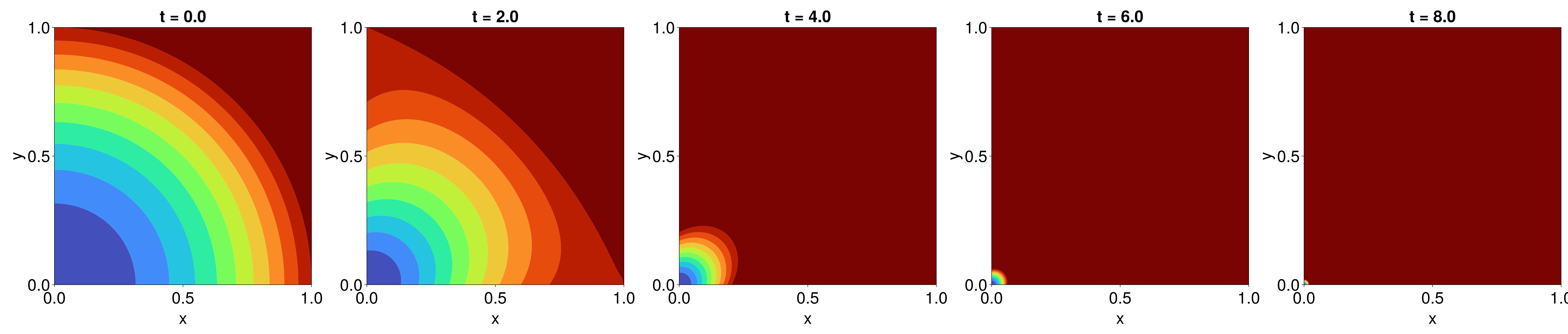

Here is how we could convert this into an FVMProblem. Note that the Neumann boundary conditions are expressed as $\grad T\vdot\vu n = 1$ above, but for FVMProblem we need them in the form $\vb q\vdot\vu n = \ldots$. For this problem, $\vb q=-D\grad T$, which gives $\vb q\vdot\vu n = -D$.

_BCs = BoundaryConditions(mesh, (x, y, t, u, p) -> -p.D(x, y, p.Dp), Neumann;
    parameters=(D=diffusion_function, Dp=diffusion_parameters))
fvm_prob = FVMProblem(
    mesh,
    _BCs;
    diffusion_function=let D=diffusion_function
        (x, y, t, u, p) -> D(x, y, p)
    end,
    diffusion_parameters=diffusion_parameters,
    source_function=let S=source_function
        (x, y, t, u, p) -> S(x, y, p) * u
    end,
    final_time=final_time,
    initial_condition=initial_condition
)
fvm_sol = solve(fvm_prob, Tsit5(), saveat=2.0)

retcode: Success
Interpolation: 1st order linear
t: 5-element Vector{Float64}:
 0.0
 2.0
 4.0
 6.0
 8.0
u: 5-element Vector{Vector{Float64}}:
 [0.0, 4.504301608035674e-5, 0.00018017206432142696, 0.00040538714472321063, 0.0007206882572857079, 0.0011260754020089186, 0.0016215485788928425, 0.0022071077879374803, 0.0028827530291428314, 0.0036484843025088956  …  1.882843115174992, 1.8955002026935723, 1.9082473762443133, 1.921084635827215, 1.9340119814422772, 1.9470294130895003, 1.9601369307688843, 1.9733345344804287, 1.986622224224134, 2.0]
 [5.392972715241152e-10, 0.0003283969313676689, 0.0012960759990657792, 0.0028772909445736296, 0.005046982038098895, 0.007780761845897453, 0.011054900287088451, 0.014846309987847455, 0.01913253192748719, 0.023891721371031495  …  1.8480635912095602, 1.8576012582610333, 1.8669187542767445, 1.8756974832998046, 1.8847639048834635, 1.8917905416460639, 1.9028817942084306, 1.9023585047422302, 1.929991725089626, 1.8825017431806468]
 [7.916735417539254e-9, 0.002394255277378073, 0.009323370071034582, 0.02042192008254062, 0.035343899135842904, 0.05376187635010671, 0.07536617230272616, 0.09986406790939101, 0.12697904481386776, 0.1564500561223998  …  1.8429322427140793, 1.8509136100103425, 1.8585916015592776, 1.8664895856726982, 1.873127291399423, 1.88258350679599, 1.884116577855119, 1.9053112112225952, 1.8762178630267217, 1.9784895515254737]
 [8.716291359760426e-8, 0.017455872288248415, 0.0670679181630476, 0.14494671157302483, 0.24751160642335912, 0.3714705521119467, 0.5138009456452608, 0.671731620222839, 0.8427259076096114, 1.0244657148949783  …  1.8491360538202182, 1.856052707050766, 1.862972930278346, 1.869629897216674, 1.8768276619393793, 1.8824054635529819, 1.8921108628658447, 1.8912414276821623, 1.9171338106695195, 1.87287270403401]
 [8.530436664276925e-7, 0.1272660020066096, 0.4824543028839799, 1.028772096825466, 1.7333054836767081, 2.5666820729791997, 3.5027585194801496, 4.51833268831315, 5.59287864642826, 6.708302802132782  …  1.8638903357448908, 1.8700526280572354, 1.8761847258134834, 1.882506501060029, 1.8884430912293937, 1.895620455128096, 1.8997922561853122, 1.9118928179026244, 1.9042195339403472, 1.948740150823866]

Using the Provided Template

The above code is implemented in LinearReactionDiffusionEquation in FiniteVolumeMethod.jl.

prob = LinearReactionDiffusionEquation(mesh, BCs;
    diffusion_function, diffusion_parameters,
    source_function,  initial_condition, final_time)
sol = solve(prob, Tsit5(); saveat=2)

retcode: Success
Interpolation: 1st order linear
t: 5-element Vector{Float64}:
 0.0
 2.0
 4.0
 6.0
 8.0
u: 5-element Vector{Vector{Float64}}:
 [0.0, 4.504301608035674e-5, 0.00018017206432142696, 0.00040538714472321063, 0.0007206882572857079, 0.0011260754020089186, 0.0016215485788928425, 0.0022071077879374803, 0.0028827530291428314, 0.0036484843025088956  …  1.8955002026935723, 1.9082473762443133, 1.921084635827215, 1.9340119814422772, 1.9470294130895003, 1.9601369307688843, 1.9733345344804287, 1.986622224224134, 2.0, 1.0]
 [5.392972715241145e-10, 0.00032839693136766827, 0.001296075999065779, 0.0028772909445736244, 0.005046982038098887, 0.007780761845897446, 0.011054900287088444, 0.014846309987847448, 0.019132531927487154, 0.023891721371031467  …  1.8576012589945818, 1.8669187520665425, 1.8756974896729597, 1.8847638872813472, 1.8917905883397685, 1.9028816744450412, 1.9023588060998364, 1.9299909590795588, 1.8825038119829294, 1.0]
 [7.916735417539239e-9, 0.0023942552773780707, 0.009323370071034585, 0.020421920082540596, 0.03534389913584282, 0.05376187635010668, 0.07536617230272617, 0.09986406790939091, 0.12697904481386757, 0.1564500561223996  …  1.8509136105141937, 1.8585916000411657, 1.866489590050211, 1.873127279309115, 1.8825835388683478, 1.8841164955936183, 1.9053114182151547, 1.876217336879789, 1.9784909725172137, 1.0]
 [8.716291359760385e-8, 0.017455872288248374, 0.0670679181630475, 0.14494671157302416, 0.24751160642335776, 0.3714705521119457, 0.5138009456452595, 0.6717316202228371, 0.8427259076096082, 1.0244657148949745  …  1.8560527056511602, 1.8629729344954407, 1.8696298850566524, 1.8768276955243501, 1.882405374461048, 1.8921110913752748, 1.8912408526896256, 1.9171352722223847, 1.872868756743993, 1.0]
 [8.530436664276848e-7, 0.1272660020066089, 0.4824543028839772, 1.0287720968254568, 1.733305483676693, 2.5666820729791855, 3.5027585194801247, 4.518332688313118, 5.592878646428218, 6.708302802132737  …  1.870052628640883, 1.8761847240549532, 1.8825065061307933, 1.8884430772243854, 1.8956204922796471, 1.8997921608963413, 1.9118930576758824, 1.9042189244693284, 1.9487417968531984, 1.0]

Here is a benchmark comparison of LinearReactionDiffusionEquation versus FVMProblem.

using BenchmarkTools
using Sundials
@btime solve($prob, $CVODE_BDF(linear_solver=:GMRES); saveat=$2);

  48.360 ms (1087 allocations: 1.58 MiB)

@btime solve($fvm_prob, $CVODE_BDF(linear_solver=:GMRES); saveat=$2);

  163.686 ms (83267 allocations: 90.84 MiB)

Just the code

An uncommented version of this example is given below. You can view the source code for this file here.

using FiniteVolumeMethod, SparseArrays, OrdinaryDiffEq, LinearAlgebra
const FVM = FiniteVolumeMethod
function linear_source_contributions!(A, mesh, conditions, source_function, source_parameters)
    for i in each_solid_vertex(mesh.triangulation)
        if !FVM.has_condition(conditions, i)
            x, y = get_point(mesh, i)
            A[i, i] += source_function(x, y, source_parameters)
        end
    end
end
function linear_reaction_diffusion_equation(mesh::FVMGeometry,
    BCs::BoundaryConditions,
    ICs::InternalConditions=InternalConditions();
    diffusion_function,
    diffusion_parameters=nothing,
    source_function,
    source_parameters=nothing,
    initial_condition,
    initial_time=0.0,
    final_time)
    conditions = Conditions(mesh, BCs, ICs)
    n = DelaunayTriangulation.num_solid_vertices(mesh.triangulation)
    Afull = zeros(n + 1, n + 1)
    A = @views Afull[begin:end-1, begin:end-1]
    b = @views Afull[begin:end-1, end]
    _ic = vcat(initial_condition, 1)
    FVM.triangle_contributions!(A, mesh, conditions, diffusion_function, diffusion_parameters)
    FVM.boundary_edge_contributions!(A, b, mesh, conditions, diffusion_function, diffusion_parameters)
    linear_source_contributions!(A, mesh, conditions, source_function, source_parameters)
    FVM.apply_dudt_conditions!(b, mesh, conditions)
    FVM.apply_dirichlet_conditions!(_ic, mesh, conditions)
    FVM.fix_missing_vertices!(A, b, mesh)
    Af = sparse(Afull)
    prob = ODEProblem(MatrixOperator(Af), _ic, (initial_time, final_time))
    return prob
end

using DelaunayTriangulation
tri = triangulate_rectangle(0, 1, 0, 1, 150, 150, single_boundary=true)
mesh = FVMGeometry(tri)
BCs = BoundaryConditions(mesh, (x, y, t, u, p) -> one(x), Neumann)
diffusion_function = (x, y, p) -> p.D * x^2 * y
diffusion_parameters = (D=1e-3,)
source_function = (x, y, p) -> (x - 1) * (y - 1)
initial_condition = [x^2 + y^2 for (x, y) in DelaunayTriangulation.each_point(tri)]
final_time = 8.0
prob = linear_reaction_diffusion_equation(mesh, BCs;
    diffusion_function, diffusion_parameters,
    source_function, initial_condition, final_time)

sol = solve(prob, Tsit5(); saveat=2)

using CairoMakie
fig = Figure(fontsize=38)
for j in eachindex(sol)
    ax = Axis(fig[1, j], width=600, height=600,
        xlabel="x", ylabel="y",
        title="t = $(sol.t[j])")
    tricontourf!(ax, tri, sol.u[j], levels=0:0.1:1, extendlow=:auto, extendhigh=:auto, colormap=:turbo)
    tightlimits!(ax)
end
resize_to_layout!(fig)
fig

_BCs = BoundaryConditions(mesh, (x, y, t, u, p) -> -p.D(x, y, p.Dp), Neumann;
    parameters=(D=diffusion_function, Dp=diffusion_parameters))
fvm_prob = FVMProblem(
    mesh,
    _BCs;
    diffusion_function=let D=diffusion_function
        (x, y, t, u, p) -> D(x, y, p)
    end,
    diffusion_parameters=diffusion_parameters,
    source_function=let S=source_function
        (x, y, t, u, p) -> S(x, y, p) * u
    end,
    final_time=final_time,
    initial_condition=initial_condition
)
fvm_sol = solve(fvm_prob, Tsit5(), saveat=2.0)

prob = LinearReactionDiffusionEquation(mesh, BCs;
    diffusion_function, diffusion_parameters,
    source_function,  initial_condition, final_time)
sol = solve(prob, Tsit5(); saveat=2)

This page was generated using Literate.jl.