Section Overview
- Section Overview
- Diffusion Equation on a Square Plate
- Diffusion Equation in a Wedge with Mixed Boundary Conditions
- Reaction Diffusion Equation with a Time-dependent Dirichlet Boundary Condition on a Disk
- Porous-Medium Equation
- Porous-Fisher Equation and Travelling Waves
- Piecewise Linear and Natural Neighbour Interpolation for an Advection-Diffusion Equation
- Helmholtz Equation with Inhomogeneous Boundary Conditions
- Laplace's Equation with Internal Dirichlet Conditions
- Equilibrium Temperature Distribution with Mixed Boundary Conditions and using EnsembleProblems
- A Reaction-Diffusion Brusselator System of PDEs
- Gray-Scott Model: Turing Patterns from a Coupled Reaction-Diffusion System
- Diffusion Equation on an Annulus
- Mean Exit Time
- Solving Mazes with Laplace's Equation
- Keller-Segel Model of Chemotaxis
We provide many tutorials in this section. Each tutorial is self-contained, although more detail will be offered in the earlier examples. At the end of each tutorial we show the uncommented code, but if you want to see the actual script itself that generates these tutorials, then click on the Edit on GitHub section on the top right of the respective tutorial.
We list all the examples below, but the tutorials can be accessed in their respective sections of the sidebar.
Note that this tutorial covers problems of the form $\partial u/\partial_t + \div\vb q = S$, and converting problems into this form. For an explanation of how to use the templates we provide for specific problems, e.g. the diffusion equation, see the Solvers for Specific Problems, and Writing Your Own section.
Diffusion Equation on a Square Plate
This tutorial considers a diffusion equation problem on a square plate:
\[\begin{equation*} \begin{aligned} \pdv{u(\vb x, t)}{t} &= \frac{1}{9}\grad^2 u(\vb x, t) & \vb x \in \Omega,\,t>0, \\[6pt] u(\vb x, t) & = 0 &\vb x \in \partial\Omega,\,t>0,\\[6pt] u(\vb x, 0) &= f(\vb x) & \vb x \in \Omega, \end{aligned} \end{equation*}\]
where $\Omega = [0, 2]^2$ and
\[f(x, y) = \begin{cases} 50 & y \leq 1, \\ 0 & y > 1. \end{cases}\]
This problem actually has an exact solution, given by[1]
\[u(\vb x, t) = \frac{200}{\pi^2}\sum_{m=1}^\infty\sum_{n=1}^\infty \frac{\left[1 + (-1)^{m+1}\right]\left[1-\cos\left(\frac{n\pi}{2}\right)\right]}{mn}\sin\left(\frac{m\pi x}{2}\right)\sin\left(\frac{n\pi y}{2}\right)\mathrm{e}^{-\frac{1}{36}\pi^2(m^2+n^2)t},\]
although we do not refer to this in the tutorial (only in the tests).
Diffusion Equation in a Wedge with Mixed Boundary Conditions
This tutorial considers a similar example as in the first example, except now the diffusion is in a wedge, has mixed boundary conditions, and is also now in polar coordinates:
\[\begin{equation*} \begin{aligned} \pdv{u(r, \theta, t)}{t} &= \grad^2u(r,\theta,t), & 0<r<1,\,0<\theta<\alpha,\,t>0,\\[6pt] \pdv{u(r, 0, t)}{\theta} & = 0 & 0<r<1,\,t>0,\\[6pt] u(1, \theta, t) &= 0 & 0<\theta<\alpha,\,t>0,\\[6pt] \pdv{u(r,\alpha,t)}{\theta} & = 0 & 0<\theta<\alpha,\,t>0,\\[6pt] u(r, \theta, 0) &= f(r,\theta) & 0<r<1,\,0<\theta<\alpha, \end{aligned} \end{equation*}\]
where we take $f(r,\theta) = 1-r$ and $\alpha=\pi/4$. This problem also has an exact solution:[2]
\[u(r, \theta, t) = \frac{1}{2}\sum_{m=1}^\infty A_{0, m}\mathrm{e}^{-\zeta_{0, m}^2t}J_0(\zeta_{0, m}r) + \sum_{n=1}^\infty\sum_{m=1}^\infty A_{n, m}\mathrm{e}^{-\zeta_{n,m}^2t}J_{n\pi/\alpha}\left(\zeta_{n\pi/\alpha,m}r\right)\cos\left(\frac{n\pi\theta}{\alpha}\right),\]
where
\[A_{n, m} = \frac{4}{\alpha J_{n\pi/\alpha+1}^2\left(\zeta_{n\pi/\alpha,m}\right)}\int_0^1\int_0^\alpha f(r, \theta)J_{n\pi/\alpha}\left(\zeta_{n\pi/\alpha,m}r\right)\cos\left(\frac{n\pi\theta}{\alpha}\right) r\dd{r}\dd{\theta}\]
for $n=0,1,2,\ldots$ and $m=1,2,3,\ldots$, and where we write the roots of $J_\mu$, the $\mu$th order Bessel function of the first kind, as $0 < \zeta_{\mu, 1} < \zeta_{\mu, 2} < \cdots$ with $\zeta_{\mu, m} \to \infty$ as $m \to \infty$. We don't discuss this in the tutorial, but it is used in the tests.
Reaction Diffusion Equation with a Time-dependent Dirichlet Boundary Condition on a Disk
This tutorial considers a reaction-diffusion problem with a $\mathrm du/\mathrm dt$ condition on a disk in polar coordinates:
\[\begin{equation*} \begin{aligned} \pdv{u(r, \theta, t)}{t} &= \div[u\grad u] + u(1-u) & 0<r<1,\,\theta<2\pi,\\[6pt] \dv{u(1, \theta, t)}{t} &= u(1,\theta,t) & 0<\theta<2\pi,\,t>0,\\[6pt] u(r,\theta,0) &= \sqrt{I_0(\sqrt{2}r)} & 0<r<1,\,0<\theta<2\pi, \end{aligned} \end{equation*}\]
where $I_0$ is the modified Bessel function of the first kind of order zero. This problem also has an exact solution,[3]
\[u(r, \theta, t) = \mathrm{e}^t\sqrt{I_0(\sqrt{2}r)}\]
that we use in the tests.
Porous-Medium Equation
This tutorial considers the porous-medium equation, given by
\[\begin{equation}\label{eq:porousmedium} \pdv{u}{t} = D\div [u^{m-1}\grad u], \end{equation}\]
with initial condition $u(\vb x, 0) = M\delta(\vb x)$ where $\delta(\vb x)$ is the Dirac delta function and $M = \iint_{\mathbb R^2} u(\vb x, t)\dd{A}$. This problem also has an exact solution that we use for defining an approximation to $\mathbb R^2$ when solving this numerically:[4]
\[\begin{equation}\label{eq:porousmediumexact} u(\vb x, t) = \begin{cases} (Dt)^{-1/m}\left[\left(\frac{M}{4\pi}\right)^{(m-1)/m}-\frac{m-1}{4m}\left(x^2+y^2\right)(Dt)^{-1/m}\right]^{1/(m-1)} & x^2+y^2 < R_{m, M}(Dt), \\ 0 & x^2+y^2 \geq R_{m, M}(Dt), \end{cases} \end{equation}\]
where $R_{m, M} = [4m/(m-1)][M/(4\pi)]^{(m-1)/m}$.
We also consider a similar problem to \eqref{eq:porousmedium}, where now the problem has a linear source:
\[\pdv{u}{t} = D\div [u^{m-1}\grad u] + \lambda u, \quad \lambda > 0,\]
which has an exact solution given by
\[u(\vb x, t) = \mathrm{e}^{\lambda t}v\left(\vb x, \frac{D}{\lambda(m-1)}\left[\mathrm{e}^{\lambda(m-1)t}-1\right]\right),\]
where $v$ is the exact solution from \eqref{eq:porousmediumexact} except with $D=1$.
Porous-Fisher Equation and Travelling Waves
This tutorial looks at the Porous-Fisher equation,
\[\begin{equation*} \begin{aligned} \pdv{u(\vb x, t)}{t} &= D \div[u\grad u] + \lambda u(1-u) & 0<x<a,\,0<y<b,\,t>0,\\[6pt] u(x, 0, t) & = 1 & 0<x<a,\,t>0,\\[6pt] u(x, b, t) & = 0 & 0<x<a,\,t>0,\\[6pt] \pdv{u(0, y, t)}{x} &= 0 & 0<y<b,\,t>0,\\[6pt] \pdv{u(a, y, t)}{x} &= 0 & 0 < y < b,\,t>0,\\[6pt] u(\vb x, 0) & = f(y) & 0 \leq x \leq a,\, 0 \leq y\leq b. \end{aligned} \end{equation*}\]
We solve this problem and also compare it to known travelling wave solutions.
Piecewise Linear and Natural Neighbour Interpolation for an Advection-Diffusion Equation
This tutorial looks at how we can apply interpolation to solutions from the PDEs discussed, making use of NaturalNeighbours.jl for this purpose. To demonstrate this, we use a two-dimensional advection equation of the form
\[\pdv{u}{t} = D\pdv[2]{u}{x} + D\pdv[2]{u}{y} - \nu\pdv{u}{x},\]
defined for $\vb x \in \mathbb R^2$ and $u(\vb x, 0) = \delta(\vb x)$, where $\delta$ is the Dirac delta function, and with homogeneous Dirichlet conditions. This problem has an exact solution, given by[5]
\[u(\vb x, t) = \frac{1}{4D\pi t}\exp\left(\frac{-(x-\nu t)^2-y^2}{4Dt}\right).\]
Helmholtz Equation with Inhomogeneous Boundary Conditions
This tutorial considers the Helmholtz equation with inhomogeneous boundary conditions:
\[\begin{equation} \begin{aligned} \grad^2 u(\vb x) + u(\vb x) &= 0 & \vb x \in [-1, 1]^2 \\ \pdv{u}{\vb n} &= 1 & \vb x \in\partial[-1,1]^2. \end{aligned} \end{equation}\]
This is different to the other problems considered thus far as the problem is now a steady state problem. The exact solution is
\[u(x, y) = -\frac{\cos(x+1)+\cos(1-x)+\cos(y+1)+\cos(1-y)}{\sin(2)}.\]
Laplace's Equation with Internal Dirichlet Conditions
This tutorial considers Laplace's equation with internal Dirichlet conditions:
\[\begin{equation} \begin{aligned} \grad^2 u &= 0 & \vb x \in [0, 1]^2, \\ u(0, y) &= 100y & 0 \leq y \leq 1, \\ u(1, y) &= 100y & 0 \leq y \leq 1, \\ u(x, 0) &= 0 & 0 \leq x \leq 1, \\ u(x, 1) &= 100 & 0 \leq x \leq 1, \\ u(1/2, y) &= 0 & 0 \leq y \leq 2/5. \end{aligned} \end{equation}\]
This last condition $u(1/2, y) = 0$ is the internal condition that needs to be dealt with.
Equilibrium Temperature Distribution with Mixed Boundary Conditions and using EnsembleProblems
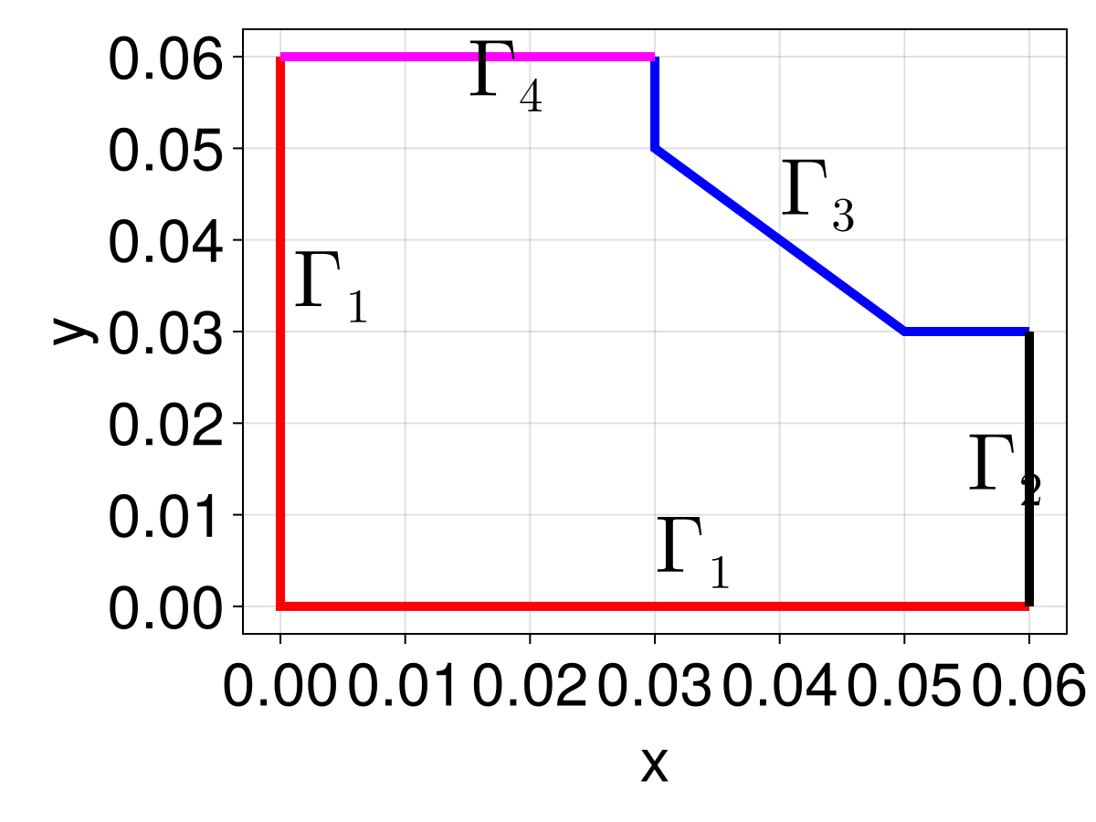
This tutorial considers the equilibrium temperature distribution in a square plate with mixed boundary conditions:
\[\begin{equation} \begin{aligned} \grad^2 T &= 0 & \vb x \in \Omega, \\ \grad T \vdot \vu n &= 0 & \vb x \in \Gamma_1, \\ T &= 40 & \vb x \in \Gamma_2, \\ k\grad T \vdot \vu n &= h(T_{\infty} - T) & \vb x \in \Gamma_3, \\ T &= 70 & \vb x \in \Gamma_4. \\ \end{aligned} \end{equation}\]
This domain $\Omega$ with boundary $\partial\Omega=\Gamma_1\cup\Gamma_2\cup\Gamma_3\cup\Gamma_4$ is shown below. For this tutorial, we also consider how varying $T_{\infty}$ affects the results, using interpolation and EnsembleProblems to study this efficiently.
A Reaction-Diffusion Brusselator System of PDEs
In this tutorial we consider the following system:
\[\begin{equation} \begin{aligned} \pdv{\Phi}{t} &= \frac14\grad^2 \Phi + \Phi^2\Psi - 2\Phi, \\ \pdv{\Psi}{t} &= \frac14\grad^2 \Psi - \Phi^2\Psi + \Phi, \end{aligned} \quad \vb x \in [0, 1]^2, \end{equation}\]
which has a solution[6]
\[\begin{equation}\label{eq:brusleexct} \begin{aligned} \Phi(x, y, t) &=\exp(-x-y-t/2), \\ \Psi(x, y, t) &= \exp(x+y+t/2). \end{aligned} \end{equation}\]
We use this exact solution to define the initial condition and Neumann boundary conditions.
Gray-Scott Model: Turing Patterns from a Coupled Reaction-Diffusion System
In this tutorial we consider the Gray-Scott model, given by
\[\begin{equation} \begin{aligned} \pdv{u}{t} &= \varepsilon_1\grad^2u+b(1-u)-uv^2, \\ \pdv{v}{t} &= \varepsilon_2\grad^2 v - dv+uv^2, \end{aligned} \end{equation}\]
with zero flux boundary conditions. We use this example to explore how changing parameters slightly leads to some amazing patterns, known as Turing patterns.[7]
Diffusion Equation on an Annulus
In this tutorial we consider the diffusion equation on an annulus:[8]
\[\begin{equation} \begin{aligned} \pdv{u(\vb x, t)}{t} &= \grad^2 u(\vb x, t) & \vb x \in \Omega, \\ \grad u(\vb x, t) \vdot \vu n(\vb x) &= 0 & \vb x \in \mathcal D(0, 1), \\ u(\vb x, t) &= c(t) & \vb x \in \mathcal D(0,0.2), \\ u(\vb x, t) &= u_0(\vb x), \end{aligned} \end{equation}\]
demonstrating how we can solve PDEs over multiply-connected domains. Here, $\mathcal D(0, r)$ is a circle of radius $r$ centered at the origin, $\Omega$ is the annulus between $\mathcal D(0,0.2)$ and $\mathcal D(0, 1)$, $c(t) = 50[1-\mathrm{e}^{-t/2}]$, and
\[u_0(x) = 10\mathrm{e}^{-25\left[\left(x+\frac12\right)^2+\left(y+\frac12\right)^2\right]} - 10\mathrm{e}^{-45\left[\left(x-\frac12\right)^2+\left(y-\frac12\right)^2\right]} - 5\mathrm{e}^{-50\left[\left(x+\frac{3}{10}\right)^2+\left(y+\frac12\right)^2\right]}.\]
We also use this tutorial as an opportunity to give an example of performing natural neighbour interpolation on a multiply-connected domain.
Mean Exit Time
In this tutorial, we consider mean time problems. The main problem we consider is that of mean exit time on a compound disk:[9]
\[\begin{equation} \begin{aligned} D_1\grad^2 T^{(1)}(\vb x) &= -1 & 0 < r < \mathcal R_1(\theta), \\ D_2\grad^2 T^{(2)}(\vb x) &= -1 & \mathcal R_1(\theta) < r < R_2(\theta), \\ T^{(1)}(\mathcal R_1(\theta),\theta) &= T^{(2)}(\mathcal R_1(\theta),\theta), \\ D_1\grad T^{(1)}(\mathcal R_1(\theta), \theta) \vdot \vu n(\theta) &= D_2\grad T^{(2)}(\mathcal R_1(\theta), \theta) \vdot \vu n(\theta), \\ T^{(2)}(R_2, \theta) &= 0, \\ \end{aligned} \end{equation}\]
with a perturbed interface $\mathcal R_1(\theta) = R_1(1+\varepsilon g(\theta))$, $g(\theta)=\sin(3\theta)+\cos(5\theta)$. The conditions at the interface are needed to enforce continuity. The variable $T^{(1)}$ is the mean exit time in $0 < r < \mathcal R_1(\theta)$, and $T^{(2)}$ is the mean exit time in $\mathcal R_1(\theta) < r < R_2(\theta)$. The end of this tutorial also considers mean exit time with obstacles and internal conditions.
Solving Mazes with Laplace's Equation
In this tutorial, we consider solving mazes using Laplace's equation, applying the result of Conolly, Burns, and Weis (1990). In particular, given a maze $\mathcal M$, represented as a collection of edges together with some starting point $\mathcal S_1$ and an endpoint $\mathcal S_2$, Laplace's equation can be used to find the solution:
\[\begin{equation} \begin{aligned} \grad^2 \phi &= 0, & \vb x \in \mathcal M, \\ \phi &= 0 & \vb x \in \mathcal S_1, \\ \phi &= 1 & \vb x \in \mathcal S_2, \\ \grad\phi\vdot\vu n &= 0 & \vb x \in \partial M \setminus (\mathcal S_1 \cup \mathcal S_2). \end{aligned} \end{equation}\]
The solution can then be found by looking at the potential $\grad\phi$.
Keller-Segel Model of Chemotaxis
In this tutorial, we consider the following Keller-Segel model of chemotaxis:[10]
\[\begin{equation*} \begin{aligned} \pdv{u}{t} &= \grad^2u - \div \left(\frac{cu}{1+u^2}\grad v\right) + u(1-u), \\ \pdv{v}{t} &= D\grad^2 v + u - av, \end{aligned} \end{equation*}\]
inside the square $[0, 100]^2$ with homogeneous Neumann boundary conditions.
- 1See here for a derivation.
- 2To derive this, use $u(r, \theta, t) = \mathrm{e}^{-\lambda t}v(r, \theta)$ and use separation of variables.
- 3See Bokhari et al. (2008) for a derivation.
- 4This exact solution is derived in Section 17.5 of the book The porous medium equation: Mathematical theory by J. L. Vázquez (2007).
- 5A derivation is given here.
- 6See Islam, Ali, and Haq (2010).
- 7There are many papers discussing this. See, e.g., Gandy and Nelson (2022) for a recent paper. The parameter values we use come from this Chebfun example.
- 8This example comes from here.
- 9This problem comes from Carr et al. (2022).
- 10This example comes from VisualPDE.