Solving Mazes with Laplace's Equation
In this tutorial, we consider solving mazes using Laplace's equation, applying the result of Conolly, Burns, and Weis (1990). In particular, given a maze $\mathcal M$, represented as a collection of edges together with some starting point $\mathcal S_1$ and an endpoint $\mathcal S_2$, Laplace's equation can be used to find the solution:
\[\begin{equation} \begin{aligned} \grad^2 \phi &= 0, & \vb x \in \mathcal M, \\ \phi &= 0 & \vb x \in \mathcal S_1, \\ \phi &= 1 & \vb x \in \mathcal S_2, \\ \grad\phi\vdot\vu n &= 0 & \vb x \in \partial M \setminus (\mathcal S_1 \cup \mathcal S_2). \end{aligned} \end{equation}\]
The gradient $\grad\phi$ will reveal the solution to the maze. We just look at $\|\grad\phi\|$ for revealing this solution, although other methods could e.g. use $\grad\phi$ to follow the associated streamlines.
Here is what the maze looks like, where the start is in blue and the end is in red.
using DelaunayTriangulation, CairoMakie, DelimitedFiles
A = readdlm(joinpath(@__DIR__, "../tutorials/maze.txt"))
A = unique(A, dims=1)
x = A[1:10:end, 2] # downsample to make the problem faster
y = A[1:10:end, 1]
start = findall(y .== 648)
finish = findall(y .== 5)
start_idx_init, start_idx_end = extrema(start)
finish_idx_init, finish_idx_end = extrema(finish)
x_start = x[start]
y_start = y[start]
x_start_to_finish = [x[start_idx_end:end]; x[begin:finish_idx_init]]
y_start_to_finish = [y[start_idx_end:end]; y[begin:finish_idx_init]]
x_finish = x[finish]
y_finish = y[finish]
x_finish_to_start = x[finish_idx_end:start_idx_init]
y_finish_to_start = y[finish_idx_end:start_idx_init]
x_bnd = [x_start, x_start_to_finish, x_finish, x_finish_to_start]
y_bnd = [y_start, y_start_to_finish, y_finish, y_finish_to_start]
boundary_nodes, points = convert_boundary_points_to_indices(x_bnd, y_bnd)
tri = triangulate(points; boundary_nodes) # takes a while because maze.txt contains so many points
refine!(tri)

fig, ax, sc, = triplot(tri,
    show_convex_hull=false,
    show_constrained_edges=false)
lines!(ax, [get_point(tri, get_boundary_nodes(tri, 1)...)...], color=:blue, linewidth=6)
lines!(ax, [get_point(tri, get_boundary_nodes(tri, 3)...)...], color=:red, linewidth=6)
fig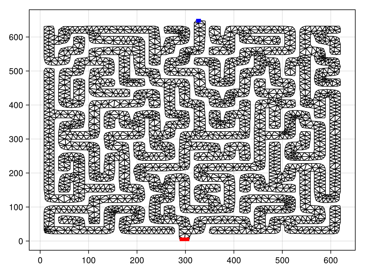
Now we can solve the problem.
using FiniteVolumeMethod, StableRNGs
mesh = FVMGeometry(tri)
start_bc = (x, y, t, u, p) -> zero(u)
start_to_finish_bc = (x, y, t, u, p) -> zero(u)
finish_bc = (x, y, t, u, p) -> one(u)
finish_to_start_bc = (x, y, t, u, p) -> zero(u)
fncs = (start_bc, start_to_finish_bc, finish_bc, finish_to_start_bc)
types = (Dirichlet, Neumann, Dirichlet, Neumann)
BCs = BoundaryConditions(mesh, fncs, types)
diffusion_function = (x, y, t, u, p) -> one(u)
initial_condition = 0.05randn(StableRNG(123), DelaunayTriangulation.num_points(tri)) # random initial condition - this is the initial guess for the solution
final_time = Inf
prob = FVMProblem(mesh, BCs;
    diffusion_function=diffusion_function,
    initial_condition=initial_condition,
    final_time=final_time)
steady_prob = SteadyFVMProblem(prob)
SteadyFVMProblem with 3824 nodesusing SteadyStateDiffEq, LinearSolve, OrdinaryDiffEq
sol = solve(steady_prob, DynamicSS(TRBDF2(linsolve=KLUFactorization(), autodiff=false)))retcode: Success
u: 3825-element Vector{Float64}:
0.0
0.0
0.00048783568415975207
0.0010463653601843787
0.001639031652859202
⋮
0.222668974705447
0.22269986424962607
0.22292603672146766
0.22330197494272958
0.05274287994504127We now have our solution.
tricontourf(tri, sol.u, colormap=:matter)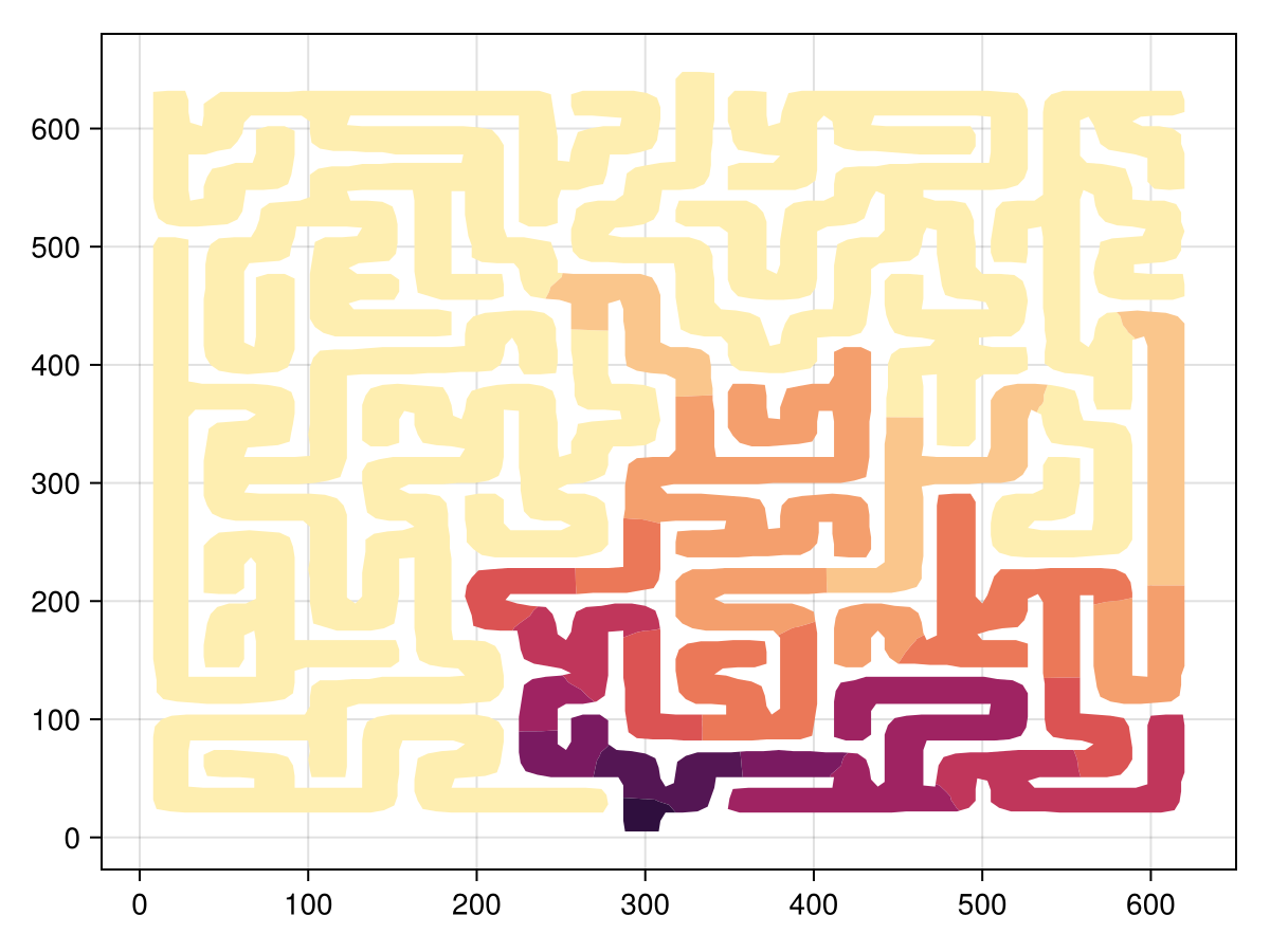
This is not what we use to compute the solution to the maze, instead we need $\grad\phi$. We compute the gradient at each point using NaturalNeighbours.jl.
using NaturalNeighbours, LinearAlgebra
itp = interpolate(tri, sol.u; derivatives=true)
∇ = NaturalNeighbours.get_gradient(itp)
∇norms = norm.(∇)
tricontourf(tri, ∇norms, colormap=:matter)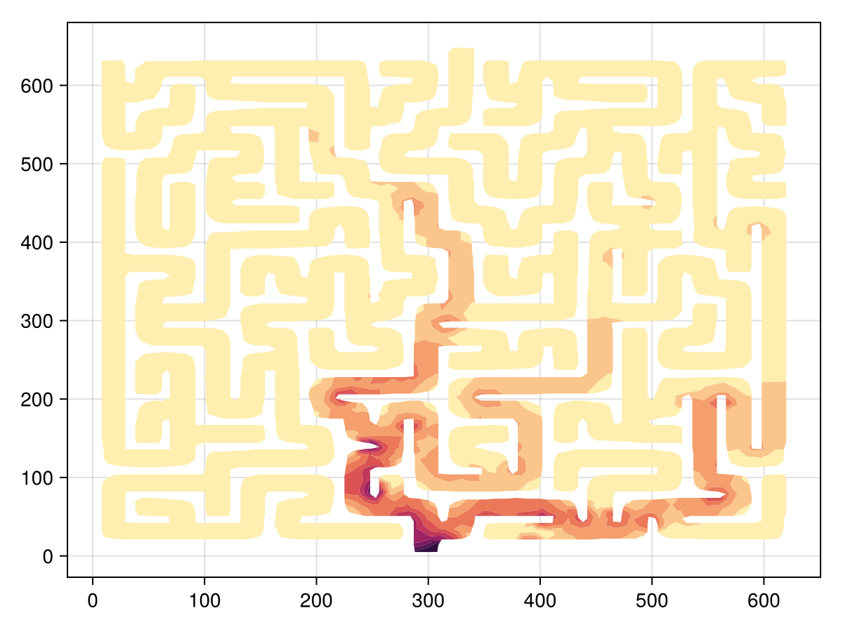
The solution to the maze is now extremely clear from this plot!
An alternative way to look at this solution is to consider the transient problem, where we do not solve the steady state problem and instead view the solution over time.
using Accessors
prob = @set prob.final_time = 1e8
LogRange(a, b, n) = exp10.(LinRange(log10(a), log10(b), n))
sol = solve(prob, TRBDF2(linsolve=KLUFactorization()), saveat=LogRange(1e2, prob.final_time, 24 * 10))
all_∇norms = map(sol.u) do u
itp = interpolate(tri, u; derivatives=true)
∇ = NaturalNeighbours.get_gradient(itp)
norm.(∇)
end
i = Observable(1)
∇norms = map(i -> all_∇norms[i], i)
fig, ax, sc = tricontourf(tri, ∇norms, colormap=:matter, levels=LinRange(0, 0.0035, 25), extendlow=:auto, extendhigh=:auto)
hidedecorations!(ax)
tightlimits!(ax)
record(fig, joinpath(@__DIR__, "../figures", "maze_solution_1.mp4"), eachindex(sol);
framerate=24) do _i
i[] = _i
end;┌ Warning: Natural neighbour interpolation is only defined over unconstrained triangulations.
│ You may find unexpected results when interpolating near the boundaries or constrained edges, and especially near non-convex boundaries or outside of the triangulation.
│ In your later evaluations of this interpolant, consider using project=false.
└ @ NaturalNeighbours ~/.julia/packages/NaturalNeighbours/HJ2P0/src/data_structures/interpolant.jl:19Just the code
An uncommented version of this example is given below. You can view the source code for this file here.
using DelaunayTriangulation, CairoMakie, DelimitedFiles
A = readdlm(joinpath(@__DIR__, "../tutorials/maze.txt"))
A = unique(A, dims=1)
x = A[1:10:end, 2] # downsample to make the problem faster
y = A[1:10:end, 1]
start = findall(y .== 648)
finish = findall(y .== 5)
start_idx_init, start_idx_end = extrema(start)
finish_idx_init, finish_idx_end = extrema(finish)
x_start = x[start]
y_start = y[start]
x_start_to_finish = [x[start_idx_end:end]; x[begin:finish_idx_init]]
y_start_to_finish = [y[start_idx_end:end]; y[begin:finish_idx_init]]
x_finish = x[finish]
y_finish = y[finish]
x_finish_to_start = x[finish_idx_end:start_idx_init]
y_finish_to_start = y[finish_idx_end:start_idx_init]
x_bnd = [x_start, x_start_to_finish, x_finish, x_finish_to_start]
y_bnd = [y_start, y_start_to_finish, y_finish, y_finish_to_start]
boundary_nodes, points = convert_boundary_points_to_indices(x_bnd, y_bnd)
tri = triangulate(points; boundary_nodes) # takes a while because maze.txt contains so many points
refine!(tri)
fig, ax, sc, = triplot(tri,
show_convex_hull=false,
show_constrained_edges=false)
lines!(ax, [get_point(tri, get_boundary_nodes(tri, 1)...)...], color=:blue, linewidth=6)
lines!(ax, [get_point(tri, get_boundary_nodes(tri, 3)...)...], color=:red, linewidth=6)
fig
using FiniteVolumeMethod, StableRNGs
mesh = FVMGeometry(tri)
start_bc = (x, y, t, u, p) -> zero(u)
start_to_finish_bc = (x, y, t, u, p) -> zero(u)
finish_bc = (x, y, t, u, p) -> one(u)
finish_to_start_bc = (x, y, t, u, p) -> zero(u)
fncs = (start_bc, start_to_finish_bc, finish_bc, finish_to_start_bc)
types = (Dirichlet, Neumann, Dirichlet, Neumann)
BCs = BoundaryConditions(mesh, fncs, types)
diffusion_function = (x, y, t, u, p) -> one(u)
initial_condition = 0.05randn(StableRNG(123), DelaunayTriangulation.num_points(tri)) # random initial condition - this is the initial guess for the solution
final_time = Inf
prob = FVMProblem(mesh, BCs;
diffusion_function=diffusion_function,
initial_condition=initial_condition,
final_time=final_time)
steady_prob = SteadyFVMProblem(prob)
using SteadyStateDiffEq, LinearSolve, OrdinaryDiffEq
sol = solve(steady_prob, DynamicSS(TRBDF2(linsolve=KLUFactorization(), autodiff=false)))
tricontourf(tri, sol.u, colormap=:matter)
using NaturalNeighbours, LinearAlgebra
itp = interpolate(tri, sol.u; derivatives=true)
∇ = NaturalNeighbours.get_gradient(itp)
∇norms = norm.(∇)
tricontourf(tri, ∇norms, colormap=:matter)
using Accessors
prob = @set prob.final_time = 1e8
LogRange(a, b, n) = exp10.(LinRange(log10(a), log10(b), n))
sol = solve(prob, TRBDF2(linsolve=KLUFactorization()), saveat=LogRange(1e2, prob.final_time, 24 * 10))
all_∇norms = map(sol.u) do u
    itp = interpolate(tri, u; derivatives=true)
    ∇ = NaturalNeighbours.get_gradient(itp)
    norm.(∇)
end
i = Observable(1)
∇norms = map(i -> all_∇norms[i], i)
fig, ax, sc = tricontourf(tri, ∇norms, colormap=:matter, levels=LinRange(0, 0.0035, 25), extendlow=:auto, extendhigh=:auto)
hidedecorations!(ax)
tightlimits!(ax)
record(fig, joinpath(@__DIR__, "../figures", "maze_solution_1.mp4"), eachindex(sol);
    framerate=24) do _i
    i[] = _i
end;This page was generated using Literate.jl.