Mean Exit Time

• Mean Exit Time
• • Definition of the problem
  • Unperturbed interface
  • Perturbed interface
  • Adding obstacles
  • Just the code

Definition of the problem

In this tutorial, we consider the problem of mean exit time, based on some of my previous work.^[1] Typically, mean exit time problems with linear diffusion take the form

\[\begin{equation}\label{eq:met} \begin{aligned} D\grad^2T(\vb x) &= -1 & \vb x \in \Omega, \\ T(\vb x) &= 0 & \vb x \in \partial \Omega, \end{aligned} \end{equation}\]

for some diffusivity $D$. $T(\vb x)$ is the mean exit time at $\vb x$, meaning the average time it would take a particle starting at $\vb x$ to exit the domain through $\partial\Omega$. For this interpretation of $T$, we are letting $D = \mathcal P\delta^2/(4\tau)$, where $\delta > 0$ is the step length of the particle, $\tau>0$ is the duration between steps, and $\mathcal P \in [0, 1]$ is the probability that the particle actually moves at a given time step.

In this previous work, we also use the finite volume method, but the problems are instead formulated as linear problems, which makes the solution significantly simpler to implement. The approach we give here is more generally applicable for other nonlinear problems, though.

A more complicated extension of \eqref{eq:met} is to allow the particle to be moving through a heterogenous media, so that the diffusivity depends on $\vb x$. In particular, let us consider a compound disk $\Omega = \{0 < r < R_1\} \cup \{R_1 < r < R_2\}$, and let $\mathcal P$ (the probability of movement) be piecewise constant across $\Omega$ (and thus also $D$):

\[P = \begin{cases} P_1 & 0<r<R_1,\\P_2&R_1<r<R_2,\end{cases}\quad D=\begin{cases}D_1&0<r<R_1,\\D_2&R_1<r<R_2,\end{cases}\]

where $D_1 = P_1\delta^2/(4\tau)$ and $D_2=P_2\delta^2/(4\tau)$. The inner region, where $0 < r < R_1$, and the outer region, where $R_1<r<R_2$, are separated by an interface at $r=R_1$ and we apply an absorbing boundary condition at $r=R_2$, meaning particles that reach $r=R_2$ exit the domain. For this problem, \eqref{eq:met} is instead given by

\[\begin{equation}\label{eq:met2} \begin{aligned} \frac{D_1}{r}\dv{r}\left(r\dv{T^{(1)}}{r}\right) &= -1 & 0 <r<R_1, \\[6pt] \frac{D_2}{r}\dv{r}\left(r\dv{T^{(2)}}{r}\right) &= -1 & R_1<r<R_2,\\[6pt] T^{(1)}(R_1) &= T^{(2)}(R_1), \\ D_1\dv{T^{(1)}}{r}(R_1) &= D_2\dv{T^{(2)}}{r}(R_1), \\[6pt] \dv{T^{(1)}}{r}(0) &= 0, \\[6pt] T^{(2)}(R_2) &= 0, \end{aligned} \end{equation}\]

which we describe using polar coordinates, and we let $T^{(1)}(r)$ be the mean exit time for $0 < r < R_1$, and $T^{(2)}(r)$ be the mean exit time for $R_1 < r < R_2$. The boundary conditions at the interface are to enforce continuity of $T$ and continuity of the flux of $T$ across the interface, and the condition $\mathrm dT^{(1)}/\mathrm dr = 0$ at $r=0$ is to ensure that $T^{(1)}$ is finite at $r=0$. This problem actually has an exact solution,

\[\begin{equation}\label{eq:met2exact} \begin{aligned} T^{(1)}(r) &= \frac{R_1^2-r^2}{4D_1}+\frac{R_2^2-R_1^2}{4D_2}, \\ T^{(2)}(r) &= \frac{R_2^2-r^2}{4D_2}, \end{aligned} \end{equation}\]

which will be useful later.

One other extension we can make is to allow the interface to be more complicated than just a circle. We take a perturbed interface, $\mathcal R_1(\theta)$, so that the inner region is now $0 < r < \mathcal R_1(\theta)$ and the outer region is $\mathcal R_1(\theta) < r < R_2$. The function $\mathcal R_1(\theta)$ is written in the form $\mathcal R_1(\theta) = R_1(1+\varepsilon g(\theta))$, where $\varepsilon \ll 1$ is a perturbation parameter, $R_1$ is the radius of the unperturbed interface, and $g(\theta)$ is a smooth $\mathcal O(1)$ periodic function with period $2\pi$; we let $g(\theta) = \sin(3\theta) + \cos(5\theta)$ and $\varepsilon=0.05$ for this tutorial. With this setup, \eqref{eq:met2} now becomes

\[\begin{equation}\label{eq:met3} \begin{aligned} D_1\grad^2 T^{(1)}(\vb x) &= -1 & 0 < r < \mathcal R_1(\theta), \\ D_2\grad^2 T^{(2)}(\vb x) &= -1 & \mathcal R_1(\theta) < r < R_2, \\ T^{(1)}(\mathcal R_1(\theta),\theta) &= T^{(2)}(\mathcal R_1(\theta),\theta), \\ D_1\grad T^{(1)}(\mathcal R_1(\theta), \theta) \vdot \vu n(\theta) &= D_2\grad T^{(2)}(\mathcal R_1(\theta), \theta) \vdot \vu n(\theta), \\ T^{(2)}(R_2, \theta) &= 0. \\ \end{aligned} \end{equation}\]

This problem has no exact solution (it has a perturbation solution, though, derived in Carr et al. (2022)).

At the end of this tutorial, we also consider modifying \eqref{eq:met3} even further so that there are holes in the domain, and an internal Dirichlet condition at the origin.

Unperturbed interface

Let us start by solving the problem on an unperturbed interface. We note that, while \eqref{eq:met2} is defined so that there are two variables $T^{(1)}$ and $T^{(2)}$, which therefore requires continuity equations across the interface, numerically we can solve this in terms of a single variable $T$ with a space-varying diffusivity. Moreover, the finiteness condition at the origin is not needed. Thus, we can solve

\[\begin{equation} \begin{aligned} D(\vb x)\grad^2 T(\vb x) &= -1 & \vb x \in \mathcal D(0, R_2), \\ T(\vb x) &= 0 & \vb x \in \partial \mathcal D(0, R_2). \end{aligned} \end{equation}\]

Here, $\mathcal D(0,R_2)$ is the circle of radius $R_2$ centred at the origin, and

\[D(\vb x) = \begin{cases} D_1 & \|\vb x\| < R_1, \\ D_2 & R_1 \leq \|\vb x\| \leq R_2. \end{cases}\]

The mesh is defined as follows. To help the accuracy of the solution, we add more triangles around the interior circle by putting some constrained edges there.

using DelaunayTriangulation, FiniteVolumeMethod, CairoMakie
R₁, R₂ = 2.0, 3.0
circle = CircularArc((0.0, R₂), (0.0, R₂), (0.0, 0.0))
points = NTuple{2,Float64}[]
tri = triangulate(points; boundary_nodes=[circle])
θ = LinRange(0, 2π, 250)
xin = @views @. R₁ * cos(θ)[begin:end-1]
yin = @views @. R₁ * sin(θ)[begin:end-1]
add_point!(tri, xin[1], yin[1])
for i in 2:length(xin)
    add_point!(tri, xin[i], yin[i])
    n = DelaunayTriangulation.num_points(tri)
    add_segment!(tri, n - 1, n)
end
n = DelaunayTriangulation.num_points(tri)
add_segment!(tri, n - 1, n)
refine!(tri; max_area=1e-3get_area(tri))
triplot(tri)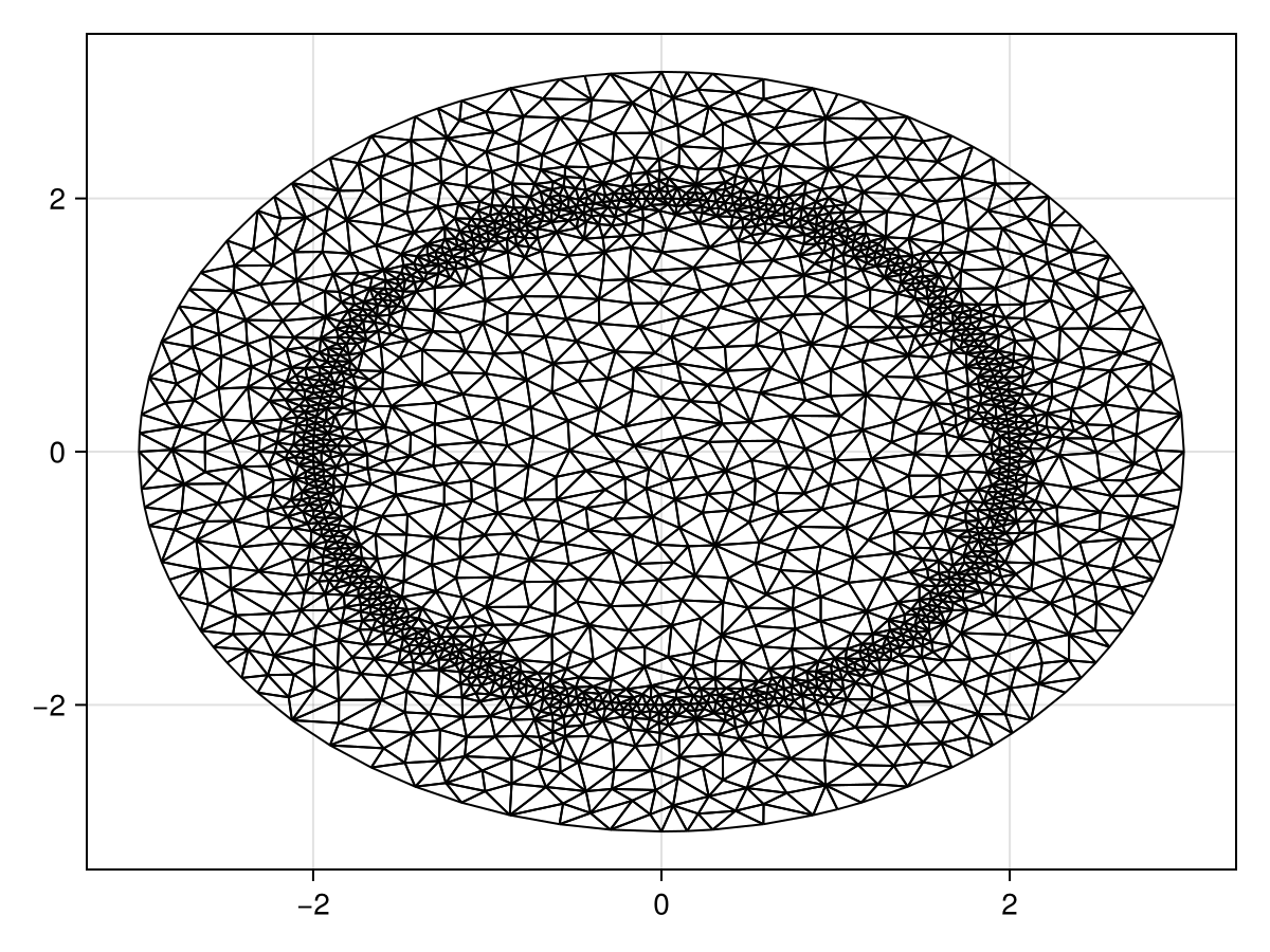

mesh = FVMGeometry(tri)

FVMGeometry with 2081 control volumes, 4068 triangles, and 6148 edges

The boundary conditions are simple absorbing conditions.

BCs = BoundaryConditions(mesh, ((x, y, t, u, p) -> zero(u),), (Dirichlet,))

BoundaryConditions with 1 boundary condition with type Dirichlet

For the problem, let us first define the diffusivity.

D₁, D₂ = 6.25e-4, 6.25e-5
diffusion_function = (x, y, t, u, p) -> let r = sqrt(x^2 + y^2)
    return ifelse(r < p.R₁, p.D₁, p.D₂)
end
diffusion_parameters = (R₁=R₁, D₁=D₁, D₂=D₂)

(R₁ = 2.0, D₁ = 0.000625, D₂ = 6.25e-5)

For the initial condition, which recall is the initial guess for the steady problem, let us use the exact solution for the mean exit time problem on a disk with a uniform diffusivity, which is given by $(R_2^2 - r^2)/(4D_2)$.

f = (x, y) -> let r = sqrt(x^2 + y^2)
    return (R₂^2 - r^2) / (4D₂)
end
initial_condition = [f(x, y) for (x, y) in DelaunayTriangulation.each_point(tri)]

2103-element Vector{Float64}:
     0.0
     0.0
     0.0
     0.0
     0.0
     ⋮
 28863.753017474664
 32730.346629636977
 27004.7281726618
 27004.728172661857
 27004.728172661886

We now define the problem.

source_function = (x, y, t, u, p) -> one(u)
prob = FVMProblem(mesh, BCs;
    diffusion_function, diffusion_parameters,
    source_function, initial_condition,
    final_time=Inf)

FVMProblem with 2081 nodes and time span (0.0, Inf)

steady_prob = SteadyFVMProblem(prob)

SteadyFVMProblem with 2081 nodes

We now solve this problem as we've done for any previous problem.

using SteadyStateDiffEq, LinearSolve, OrdinaryDiffEq
sol = solve(steady_prob, DynamicSS(Rosenbrock23()))

retcode: Success
u: 2103-element Vector{Float64}:
     0.0
     0.0
     0.0
     0.0
     0.0
     ⋮
 21207.486988380246
 21600.970814671047
 21016.51514820288
 21016.16928985875
 21016.403266543497

fig = Figure(fontsize=33)
ax = Axis(fig[1, 1], xlabel="x", ylabel="y")
tricontourf!(ax, tri, sol.u, levels=0:500:20000, extendhigh=:auto)
fig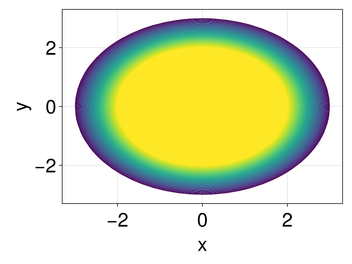

Perturbed interface

Let us now solve the problem with a perturbed interface. The mesh is defined as follows.

g = θ -> sin(3θ) + cos(5θ)
ε = 0.05
R1_f = θ -> R₁ * (1 + ε * g(θ))
points = NTuple{2,Float64}[]
circle = CircularArc((0.0, R₂), (0.0, R₂), (0.0, 0.0))
tri = triangulate(points; boundary_nodes=[circle])
xin = @views (@. R1_f(θ) * cos(θ))[begin:end-1]
yin = @views (@. R1_f(θ) * sin(θ))[begin:end-1]
add_point!(tri, xin[1], yin[1])
for i in 2:length(xin)
    add_point!(tri, xin[i], yin[i])
    n = DelaunayTriangulation.num_points(tri)
    add_segment!(tri, n - 1, n)
end
n = DelaunayTriangulation.num_points(tri)
add_segment!(tri, n - 1, n)
refine!(tri; max_area=1e-3get_area(tri))
triplot(tri)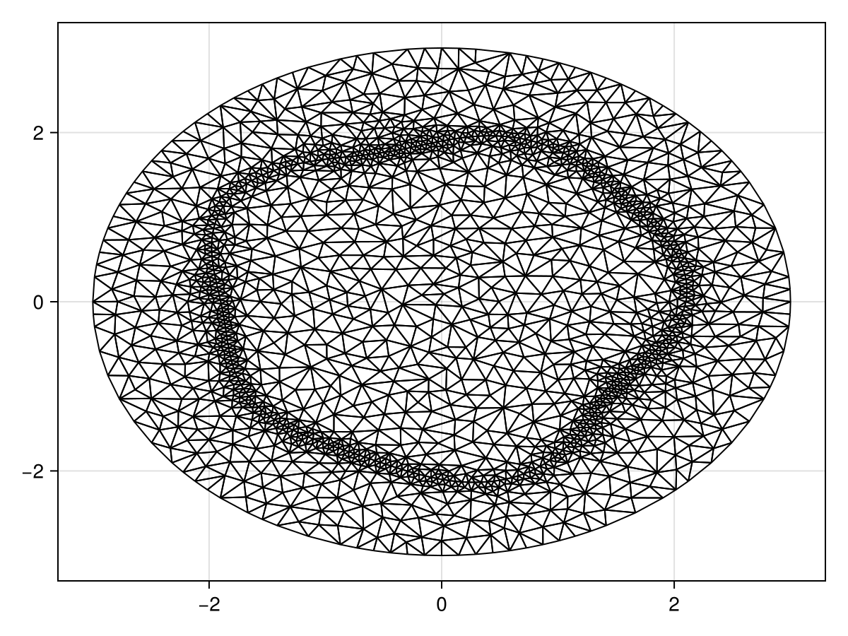

mesh = FVMGeometry(tri)

FVMGeometry with 1864 control volumes, 3623 triangles, and 5486 edges

The boundary conditions are simple absorbing conditions.

BCs = BoundaryConditions(mesh, (x, y, t, u, p) -> zero(u), Dirichlet)

BoundaryConditions with 1 boundary condition with type Dirichlet

Now we define the problem. For the initial condition that we use, we will use the exact solution for the problem with an unperturbed interface.

function T_exact(x, y)
    r = sqrt(x^2 + y^2)
    if r < R₁
        return (R₁^2 - r^2) / (4D₁) + (R₂^2 - R₁^2) / (4D₂)
    else
        return (R₂^2 - r^2) / (4D₂)
    end
end
diffusion_function = (x, y, t, u, p) -> let r = sqrt(x^2 + y^2), θ = atan(y, x)
    interface_val = p.R1_f(θ)
    return ifelse(r < interface_val, p.D₁, p.D₂)
end
diffusion_parameters = (D₁=D₁, D₂=D₂, R1_f=R1_f)
initial_condition = [T_exact(x, y) for (x, y) in DelaunayTriangulation.each_point(tri)]
source_function = (x, y, t, u, p) -> one(u)
prob = FVMProblem(mesh, BCs;
    diffusion_function, diffusion_parameters,
    source_function, initial_condition,
    final_time=Inf)
steady_prob = SteadyFVMProblem(prob)

SteadyFVMProblem with 1864 nodes

sol = solve(steady_prob, DynamicSS(Rosenbrock23()))

retcode: Success
u: 1898-element Vector{Float64}:
    0.0
    0.0
    0.0
    0.0
    0.0
    ⋮
 8237.434881424284
 6812.802679524329
 3382.053786112592
 3706.2254680231426
 3462.5064362649373

fig = Figure(fontsize=33)
ax = Axis(fig[1, 1], xlabel="x", ylabel="y")
tricontourf!(ax, tri, sol.u, levels=0:500:20000, extendhigh=:auto)
lines!(ax, [xin; xin[1]], [yin; yin[1]], color=:magenta, linewidth=5)
fig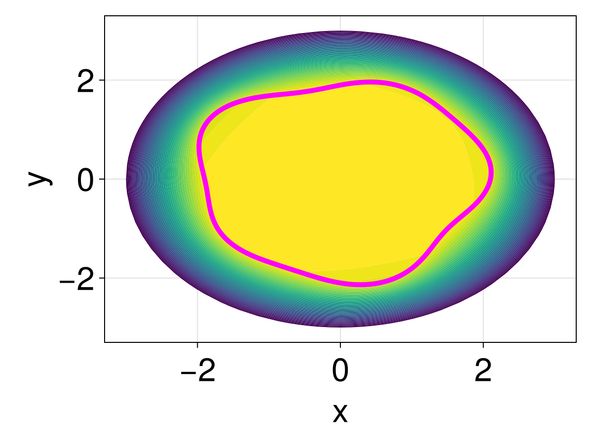

Adding obstacles

Let us now add some obstacles into the problem. We add in components one at a time, exploring the impact of each component individually. When we update the triangulation, we do need to update the mesh since it is constructed from the initial tri.

The first obstacle we consider adding is a single hole at the origin, which we accomplish by adding a point at the origin and then using InternalConditions. This point will be used to absorb any nearby particles, i.e. $T(0,0)=0$.

add_point!(tri, 0.0, 0.0)
mesh = FVMGeometry(tri)
ICs = InternalConditions((x, y, t, u, p) -> zero(u), dirichlet_nodes=Dict(DelaunayTriangulation.num_points(tri) => 1))
BCs = BoundaryConditions(mesh, (x, y, t, u, p) -> zero(u), Dirichlet)
initial_condition = [T_exact(x, y) for (x, y) in DelaunayTriangulation.each_point(tri)]
prob = FVMProblem(mesh, BCs, ICs;
    diffusion_function, diffusion_parameters,
    source_function, initial_condition,
    final_time=Inf)
steady_prob = SteadyFVMProblem(prob)
sol = solve(steady_prob, DynamicSS(Rosenbrock23()))
fig = Figure(fontsize=33)
ax = Axis(fig[1, 1], xlabel="x", ylabel="y")
tricontourf!(ax, tri, sol.u, levels=0:500:10000, extendhigh=:auto)
lines!(ax, [xin; xin[1]], [yin; yin[1]], color=:magenta, linewidth=5)
fig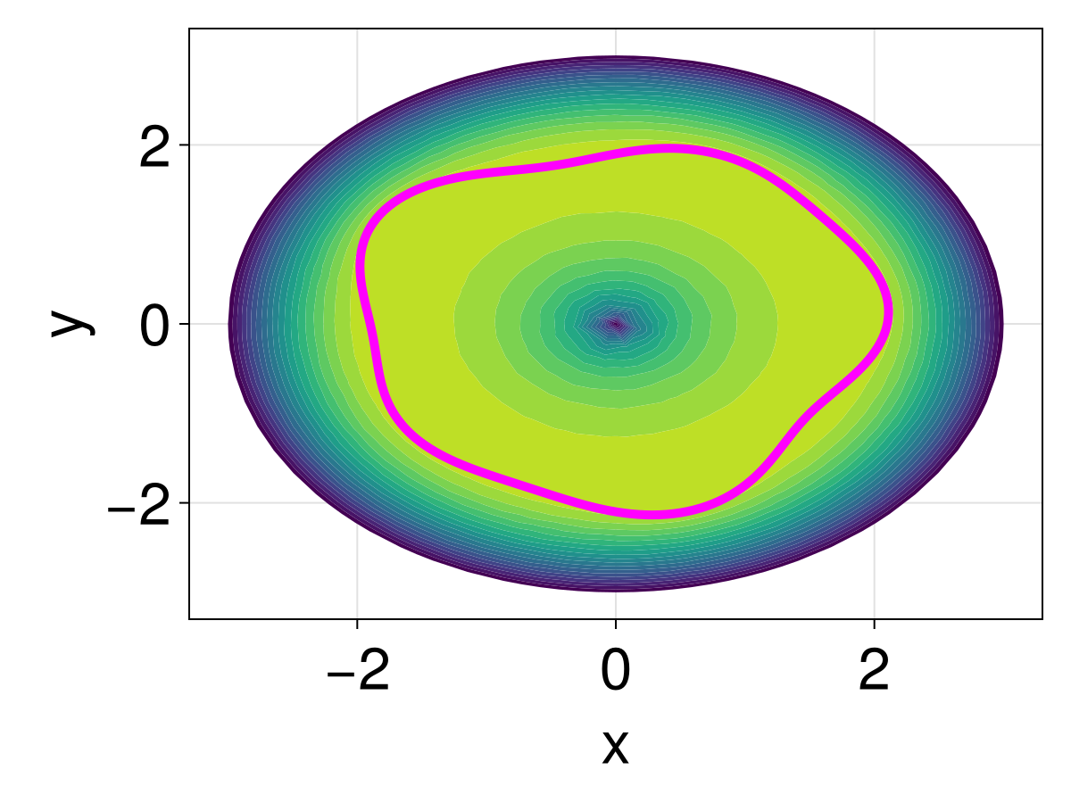

We see that the hole has changed the interior significantly. For the next constraint, let us change the boundary so that we only allow particles to exit through a small part of the boundary, reflecting off all other parts. For the reflecting boundary condition, this is enforced by using Neumann boundary conditions.

ϵr = 0.25
dirichlet_circle = CircularArc((R₂ * cos(ϵr), R₂ * sin(ϵr)), (R₂ * cos(2π - ϵr), R₂ * sin(2π - ϵr)), (0.0, 0.0))
neumann_circle = CircularArc((R₂ * cos(2π - ϵr), R₂ * sin(2π - ϵr)), (R₂ * cos(ϵr), R₂ * sin(ϵr)), (0.0, 0.0))
boundary_nodes = [[dirichlet_circle], [neumann_circle]]
points = NTuple{2,Float64}[]
tri = triangulate(points; boundary_nodes)
xin = @views (@. R1_f(θ) * cos(θ))[begin:end-1]
yin = @views (@. R1_f(θ) * sin(θ))[begin:end-1]
add_point!(tri, xin[1], yin[1])
for i in 2:length(xin)
    add_point!(tri, xin[i], yin[i])
    n = DelaunayTriangulation.num_points(tri)
    add_segment!(tri, n - 1, n)
end
n = DelaunayTriangulation.num_points(tri)
add_segment!(tri, n - 1, n)
add_point!(tri, 0.0, 0.0)
origin_idx = DelaunayTriangulation.num_points(tri)
refine!(tri; max_area=1e-3get_area(tri))
triplot(tri)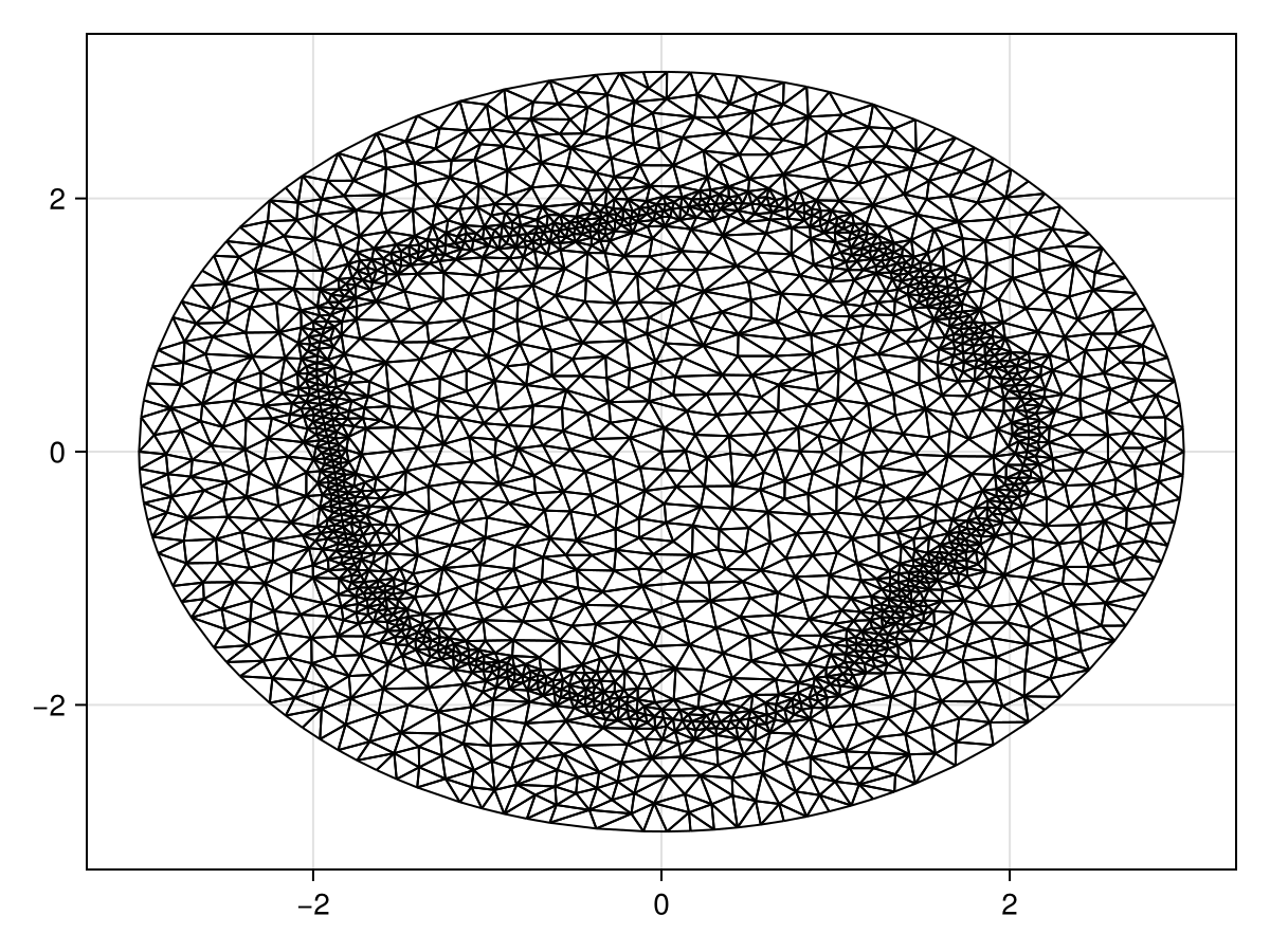

mesh = FVMGeometry(tri)
zero_f = (x, y, t, u, p) -> zero(u)
BCs = BoundaryConditions(mesh, (zero_f, zero_f), (Neumann, Dirichlet))
ICs = InternalConditions((x, y, t, u, p) -> zero(u), dirichlet_nodes=Dict(origin_idx => 1))
initial_condition = [T_exact(x, y) for (x, y) in DelaunayTriangulation.each_point(tri)]
prob = FVMProblem(mesh, BCs, ICs;
    diffusion_function, diffusion_parameters,
    source_function, initial_condition,
    final_time=Inf)
steady_prob = SteadyFVMProblem(prob)
sol = solve(steady_prob, DynamicSS(Rosenbrock23()))
fig = Figure(fontsize=33)
ax = Axis(fig[1, 1], xlabel="x", ylabel="y")
tricontourf!(ax, tri, sol.u, levels=0:2500:35000, extendhigh=:auto)
lines!(ax, [xin; xin[1]], [yin; yin[1]], color=:magenta, linewidth=5)
fig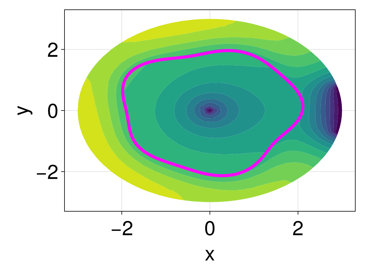

Now, as a last constraint, let's add a hole. We'll put hole at the origin, and we'll move the point hole to $(-2, 0)$ rather than at the origin, and we'll also put a hole at $(0, 2.95)$.

hole = CircularArc((0.0, 1.0), (0.0, 1.0), (0.0, 0.0), positive=false)
boundary_nodes = [[[dirichlet_circle], [neumann_circle]], [[hole]]]
points = NTuple{2,Float64}[]
tri = triangulate(points; boundary_nodes)
xin = @views (@. R1_f(θ) * cos(θ))[begin:end-1]
yin = @views (@. R1_f(θ) * sin(θ))[begin:end-1]
add_point!(tri, xin[1], yin[1])
for i in 2:length(xin)
    add_point!(tri, xin[i], yin[i])
    n = DelaunayTriangulation.num_points(tri)
    add_segment!(tri, n - 1, n)
end
n = DelaunayTriangulation.num_points(tri)
add_segment!(tri, n - 1, n)
add_point!(tri, -2.0, 0.0)
add_point!(tri, 0.0, 2.95)
pointhole_idxs = [DelaunayTriangulation.num_points(tri), DelaunayTriangulation.num_points(tri) - 1]
refine!(tri; max_area=1e-3get_area(tri))
triplot(tri)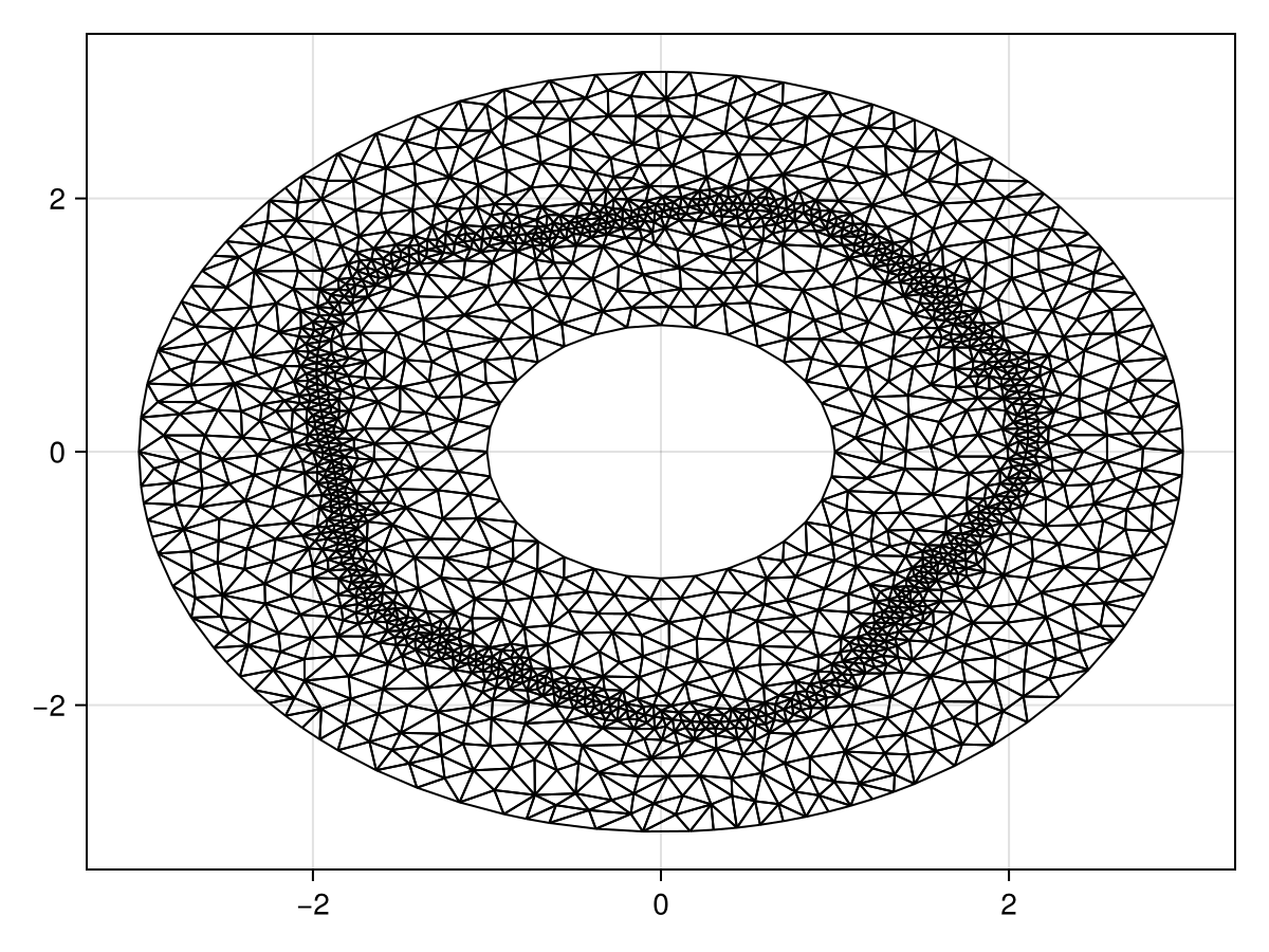

The boundary condition we'll use at the new interior hole will be an absorbing boundary condition.

mesh = FVMGeometry(tri)
zero_f = (x, y, t, u, p) -> zero(u)
BCs = BoundaryConditions(mesh, (zero_f, zero_f, zero_f), (Neumann, Dirichlet, Dirichlet))
ICs = InternalConditions((x, y, t, u, p) -> zero(u), dirichlet_nodes=Dict(pointhole_idxs .=> 1))
initial_condition = [T_exact(x, y) for (x, y) in DelaunayTriangulation.each_point(tri)]
prob = FVMProblem(mesh, BCs, ICs;
    diffusion_function, diffusion_parameters,
    source_function, initial_condition,
    final_time=Inf)
steady_prob = SteadyFVMProblem(prob)
sol = solve(steady_prob, DynamicSS(Rosenbrock23()))
fig = Figure(fontsize=33)
ax = Axis(fig[1, 1], xlabel="x", ylabel="y")
tricontourf!(ax, tri, sol.u, levels=0:1000:15000, extendhigh=:auto)
lines!(ax, [xin; xin[1]], [yin; yin[1]], color=:magenta, linewidth=5)
fig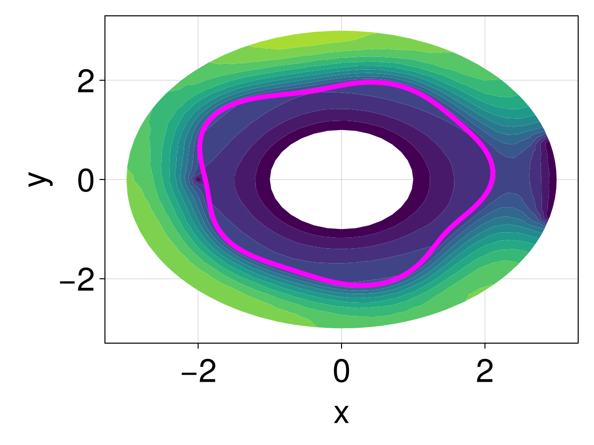

Just the code

An uncommented version of this example is given below. You can view the source code for this file here.

using DelaunayTriangulation, FiniteVolumeMethod, CairoMakie
R₁, R₂ = 2.0, 3.0
circle = CircularArc((0.0, R₂), (0.0, R₂), (0.0, 0.0))
points = NTuple{2,Float64}[]
tri = triangulate(points; boundary_nodes=[circle])
θ = LinRange(0, 2π, 250)
xin = @views @. R₁ * cos(θ)[begin:end-1]
yin = @views @. R₁ * sin(θ)[begin:end-1]
add_point!(tri, xin[1], yin[1])
for i in 2:length(xin)
    add_point!(tri, xin[i], yin[i])
    n = DelaunayTriangulation.num_points(tri)
    add_segment!(tri, n - 1, n)
end
n = DelaunayTriangulation.num_points(tri)
add_segment!(tri, n - 1, n)
refine!(tri; max_area=1e-3get_area(tri))
triplot(tri)

mesh = FVMGeometry(tri)

BCs = BoundaryConditions(mesh, ((x, y, t, u, p) -> zero(u),), (Dirichlet,))

D₁, D₂ = 6.25e-4, 6.25e-5
diffusion_function = (x, y, t, u, p) -> let r = sqrt(x^2 + y^2)
    return ifelse(r < p.R₁, p.D₁, p.D₂)
end
diffusion_parameters = (R₁=R₁, D₁=D₁, D₂=D₂)

f = (x, y) -> let r = sqrt(x^2 + y^2)
    return (R₂^2 - r^2) / (4D₂)
end
initial_condition = [f(x, y) for (x, y) in DelaunayTriangulation.each_point(tri)]

source_function = (x, y, t, u, p) -> one(u)
prob = FVMProblem(mesh, BCs;
    diffusion_function, diffusion_parameters,
    source_function, initial_condition,
    final_time=Inf)

steady_prob = SteadyFVMProblem(prob)

using SteadyStateDiffEq, LinearSolve, OrdinaryDiffEq
sol = solve(steady_prob, DynamicSS(Rosenbrock23()))

fig = Figure(fontsize=33)
ax = Axis(fig[1, 1], xlabel="x", ylabel="y")
tricontourf!(ax, tri, sol.u, levels=0:500:20000, extendhigh=:auto)
fig

g = θ -> sin(3θ) + cos(5θ)
ε = 0.05
R1_f = θ -> R₁ * (1 + ε * g(θ))
points = NTuple{2,Float64}[]
circle = CircularArc((0.0, R₂), (0.0, R₂), (0.0, 0.0))
tri = triangulate(points; boundary_nodes=[circle])
xin = @views (@. R1_f(θ) * cos(θ))[begin:end-1]
yin = @views (@. R1_f(θ) * sin(θ))[begin:end-1]
add_point!(tri, xin[1], yin[1])
for i in 2:length(xin)
    add_point!(tri, xin[i], yin[i])
    n = DelaunayTriangulation.num_points(tri)
    add_segment!(tri, n - 1, n)
end
n = DelaunayTriangulation.num_points(tri)
add_segment!(tri, n - 1, n)
refine!(tri; max_area=1e-3get_area(tri))
triplot(tri)

mesh = FVMGeometry(tri)

BCs = BoundaryConditions(mesh, (x, y, t, u, p) -> zero(u), Dirichlet)

function T_exact(x, y)
    r = sqrt(x^2 + y^2)
    if r < R₁
        return (R₁^2 - r^2) / (4D₁) + (R₂^2 - R₁^2) / (4D₂)
    else
        return (R₂^2 - r^2) / (4D₂)
    end
end
diffusion_function = (x, y, t, u, p) -> let r = sqrt(x^2 + y^2), θ = atan(y, x)
    interface_val = p.R1_f(θ)
    return ifelse(r < interface_val, p.D₁, p.D₂)
end
diffusion_parameters = (D₁=D₁, D₂=D₂, R1_f=R1_f)
initial_condition = [T_exact(x, y) for (x, y) in DelaunayTriangulation.each_point(tri)]
source_function = (x, y, t, u, p) -> one(u)
prob = FVMProblem(mesh, BCs;
    diffusion_function, diffusion_parameters,
    source_function, initial_condition,
    final_time=Inf)
steady_prob = SteadyFVMProblem(prob)

sol = solve(steady_prob, DynamicSS(Rosenbrock23()))

fig = Figure(fontsize=33)
ax = Axis(fig[1, 1], xlabel="x", ylabel="y")
tricontourf!(ax, tri, sol.u, levels=0:500:20000, extendhigh=:auto)
lines!(ax, [xin; xin[1]], [yin; yin[1]], color=:magenta, linewidth=5)
fig

add_point!(tri, 0.0, 0.0)
mesh = FVMGeometry(tri)
ICs = InternalConditions((x, y, t, u, p) -> zero(u), dirichlet_nodes=Dict(DelaunayTriangulation.num_points(tri) => 1))
BCs = BoundaryConditions(mesh, (x, y, t, u, p) -> zero(u), Dirichlet)
initial_condition = [T_exact(x, y) for (x, y) in DelaunayTriangulation.each_point(tri)]
prob = FVMProblem(mesh, BCs, ICs;
    diffusion_function, diffusion_parameters,
    source_function, initial_condition,
    final_time=Inf)
steady_prob = SteadyFVMProblem(prob)
sol = solve(steady_prob, DynamicSS(Rosenbrock23()))
fig = Figure(fontsize=33)
ax = Axis(fig[1, 1], xlabel="x", ylabel="y")
tricontourf!(ax, tri, sol.u, levels=0:500:10000, extendhigh=:auto)
lines!(ax, [xin; xin[1]], [yin; yin[1]], color=:magenta, linewidth=5)
fig

ϵr = 0.25
dirichlet_circle = CircularArc((R₂ * cos(ϵr), R₂ * sin(ϵr)), (R₂ * cos(2π - ϵr), R₂ * sin(2π - ϵr)), (0.0, 0.0))
neumann_circle = CircularArc((R₂ * cos(2π - ϵr), R₂ * sin(2π - ϵr)), (R₂ * cos(ϵr), R₂ * sin(ϵr)), (0.0, 0.0))
boundary_nodes = [[dirichlet_circle], [neumann_circle]]
points = NTuple{2,Float64}[]
tri = triangulate(points; boundary_nodes)
xin = @views (@. R1_f(θ) * cos(θ))[begin:end-1]
yin = @views (@. R1_f(θ) * sin(θ))[begin:end-1]
add_point!(tri, xin[1], yin[1])
for i in 2:length(xin)
    add_point!(tri, xin[i], yin[i])
    n = DelaunayTriangulation.num_points(tri)
    add_segment!(tri, n - 1, n)
end
n = DelaunayTriangulation.num_points(tri)
add_segment!(tri, n - 1, n)
add_point!(tri, 0.0, 0.0)
origin_idx = DelaunayTriangulation.num_points(tri)
refine!(tri; max_area=1e-3get_area(tri))
triplot(tri)

mesh = FVMGeometry(tri)
zero_f = (x, y, t, u, p) -> zero(u)
BCs = BoundaryConditions(mesh, (zero_f, zero_f), (Neumann, Dirichlet))
ICs = InternalConditions((x, y, t, u, p) -> zero(u), dirichlet_nodes=Dict(origin_idx => 1))
initial_condition = [T_exact(x, y) for (x, y) in DelaunayTriangulation.each_point(tri)]
prob = FVMProblem(mesh, BCs, ICs;
    diffusion_function, diffusion_parameters,
    source_function, initial_condition,
    final_time=Inf)
steady_prob = SteadyFVMProblem(prob)
sol = solve(steady_prob, DynamicSS(Rosenbrock23()))
fig = Figure(fontsize=33)
ax = Axis(fig[1, 1], xlabel="x", ylabel="y")
tricontourf!(ax, tri, sol.u, levels=0:2500:35000, extendhigh=:auto)
lines!(ax, [xin; xin[1]], [yin; yin[1]], color=:magenta, linewidth=5)
fig

hole = CircularArc((0.0, 1.0), (0.0, 1.0), (0.0, 0.0), positive=false)
boundary_nodes = [[[dirichlet_circle], [neumann_circle]], [[hole]]]
points = NTuple{2,Float64}[]
tri = triangulate(points; boundary_nodes)
xin = @views (@. R1_f(θ) * cos(θ))[begin:end-1]
yin = @views (@. R1_f(θ) * sin(θ))[begin:end-1]
add_point!(tri, xin[1], yin[1])
for i in 2:length(xin)
    add_point!(tri, xin[i], yin[i])
    n = DelaunayTriangulation.num_points(tri)
    add_segment!(tri, n - 1, n)
end
n = DelaunayTriangulation.num_points(tri)
add_segment!(tri, n - 1, n)
add_point!(tri, -2.0, 0.0)
add_point!(tri, 0.0, 2.95)
pointhole_idxs = [DelaunayTriangulation.num_points(tri), DelaunayTriangulation.num_points(tri) - 1]
refine!(tri; max_area=1e-3get_area(tri))
triplot(tri)

mesh = FVMGeometry(tri)
zero_f = (x, y, t, u, p) -> zero(u)
BCs = BoundaryConditions(mesh, (zero_f, zero_f, zero_f), (Neumann, Dirichlet, Dirichlet))
ICs = InternalConditions((x, y, t, u, p) -> zero(u), dirichlet_nodes=Dict(pointhole_idxs .=> 1))
initial_condition = [T_exact(x, y) for (x, y) in DelaunayTriangulation.each_point(tri)]
prob = FVMProblem(mesh, BCs, ICs;
    diffusion_function, diffusion_parameters,
    source_function, initial_condition,
    final_time=Inf)
steady_prob = SteadyFVMProblem(prob)
sol = solve(steady_prob, DynamicSS(Rosenbrock23()))
fig = Figure(fontsize=33)
ax = Axis(fig[1, 1], xlabel="x", ylabel="y")
tricontourf!(ax, tri, sol.u, levels=0:1000:15000, extendhigh=:auto)
lines!(ax, [xin; xin[1]], [yin; yin[1]], color=:magenta, linewidth=5)
fig

This page was generated using Literate.jl.