Laplace's Equation

Laplace's Equation

Now we consider Laplace's equation. What we produce in this section can also be accessed in FiniteVolumeMethod.LaplacesEquation.

Mathematical Details

The mathematical details for this solver are the same as for our Poisson equation example, except with $f = 0$. The problems being solved are of the form

\[\div\left[D(\vb x)\grad u\right] = 0,\]

known as the generalised Laplace equation.^[1]

Implementation

For the implementation, we can reuse a lot of what we had for Poisson's equation, except that we don't need create_rhs_b.

using FiniteVolumeMethod, SparseArrays, DelaunayTriangulation, LinearSolve
const FVM = FiniteVolumeMethod
function laplaces_equation(mesh::FVMGeometry,
    BCs::BoundaryConditions,
    ICs::InternalConditions=InternalConditions();
    diffusion_function=(x, y, p) -> 1.0,
    diffusion_parameters=nothing)
    conditions = Conditions(mesh, BCs, ICs)
    n = DelaunayTriangulation.num_points(mesh.triangulation)
    A = zeros(n, n)
    b = zeros(DelaunayTriangulation.num_points(mesh.triangulation))
    FVM.triangle_contributions!(A, mesh, conditions, diffusion_function, diffusion_parameters)
    FVM.boundary_edge_contributions!(A, b, mesh, conditions, diffusion_function, diffusion_parameters)
    FVM.apply_steady_dirichlet_conditions!(A, b, mesh, conditions)
    FVM.fix_missing_vertices!(A, b, mesh)
    Asp = sparse(A)
    prob = LinearProblem(Asp, b)
    return prob
end

laplaces_equation (generic function with 2 methods)

Now let's test this problem. We consider Laplace's equation on a sector of an annulus, so that^[2]

\[\begin{equation*} \begin{aligned} \grad^2 u &= 1 < r > 2,\,0 < \theta < \pi/2, \\ u(x, 0) &= 0 & 1 < x < 2, \\ u(0, y) &= 0 & 1 < y < 2, \\ u(x, y) &= 2xy & r = 1, \\ u(x, y) &= \left(\frac{\pi}{2} - \arctan\frac{y}{x}\right)\arctan\frac{y}{x} & r = 2. \end{aligned} \end{equation*}\]

To start, we define our mesh. We need to define each part of the annulus separately, which takes some care.

using CairoMakie
lower_x = [1.0, 2.0]
lower_y = [0.0, 0.0]
θ = LinRange(0, π / 2, 100)
outer_arc_x = 2cos.(θ)
outer_arc_x[end] = 0.0 # must match with left_x
outer_arc_y = 2sin.(θ)
left_x = [0.0, 0.0]
left_y = [2.0, 1.0]
inner_arc_x = cos.(θ) |> reverse!
inner_arc_x[begin] = 0.0 # must match with left_x
inner_arc_y = sin.(θ) |> reverse!
boundary_x = [lower_x, outer_arc_x, left_x, inner_arc_x]
boundary_y = [lower_y, outer_arc_y, left_y, inner_arc_y]
boundary_nodes, points = convert_boundary_points_to_indices(boundary_x, boundary_y)
tri = triangulate(points; boundary_nodes)
refine!(tri; max_area=1e-3get_area(tri))
triplot(tri)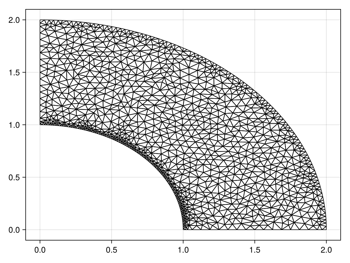

mesh = FVMGeometry(tri)

FVMGeometry with 1204 control volumes, 2169 triangles, and 3372 edges

The boundary conditions are defined as follows.

lower_f = (x, y, t, u, p) -> 0.0
outer_arc_f = (x, y, t, u, p) -> (π / 2 - atan(y, x)) * atan(y, x)
left_f = (x, y, t, u, p) -> 2x * y
inner_arc_f = (x, y, t, u, p) -> 2x * y
bc_f = (lower_f, outer_arc_f, left_f, inner_arc_f)
bc_types = (Dirichlet, Dirichlet, Dirichlet, Dirichlet)
BCs = BoundaryConditions(mesh, bc_f, bc_types)

BoundaryConditions with 4 boundary conditions with types (Dirichlet, Dirichlet, Dirichlet, Dirichlet)

Now we can define and solve the problem.

prob = laplaces_equation(mesh, BCs, diffusion_function=(x, y, p) -> 1.0)

LinearProblem. In-place: true
b: 1218-element Vector{Float64}:
 0.0
 0.0
 0.024671493503386318
 0.04883948713935658
 0.0725039809079108
 ⋮
 0.0
 0.0
 0.0
 0.0
 0.0

sol = solve(prob, KLUFactorization())

retcode: Default
u: 1218-element Vector{Float64}:
 0.0
 0.0
 0.024671493503386318
 0.04883948713935658
 0.0725039809079108
 ⋮
 0.6366323481213669
 0.5030201436106874
 0.11918344183907012
 0.18232094714968392
 0.18279310176598018

fig = Figure(fontsize=33)
ax = Axis(fig[1, 1], xlabel="x", ylabel="y", width=600, height=600)
tricontourf!(ax, tri, sol.u, levels=0:0.1:1, colormap=:jet)
resize_to_layout!(fig)
fig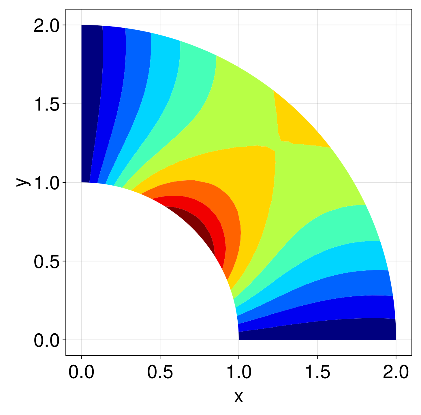

We can turn this type of problem into its corresponding SteadyFVMProblem as follows:

initial_condition = zeros(DelaunayTriangulation.num_points(tri))
FVM.apply_dirichlet_conditions!(initial_condition, mesh, Conditions(mesh, BCs, InternalConditions())) # a good initial guess
fvm_prob = SteadyFVMProblem(FVMProblem(mesh, BCs;
    diffusion_function=(x, y, t, u, p) -> 1.0,
    initial_condition,
    final_time=Inf))

SteadyFVMProblem with 1204 nodes

using SteadyStateDiffEq, OrdinaryDiffEq
fvm_sol = solve(fvm_prob, DynamicSS(TRBDF2()))

retcode: Success
u: 1218-element Vector{Float64}:
 0.0
 0.0
 0.024671493503386318
 0.04883948713935658
 0.0725039809079108
 ⋮
 0.6366323292638485
 0.5030201298661489
 0.11918343865285634
 0.18232094165591534
 0.18279309684361356

ax = Axis(fig[1, 2], xlabel="x", ylabel="y", width=600, height=600)
tricontourf!(ax, tri, fvm_sol.u, levels=0:0.1:1, colormap=:jet)
resize_to_layout!(fig)
fig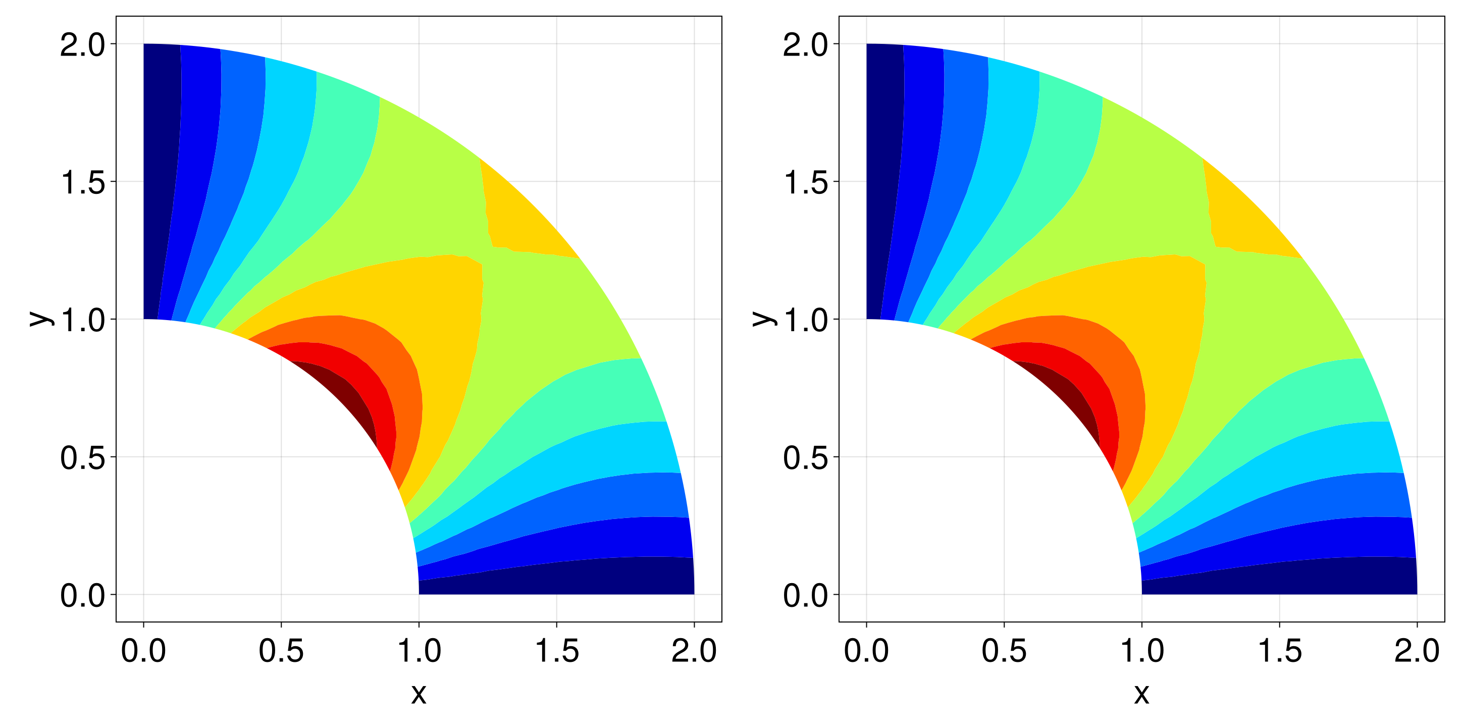

Using the Provided Template

Let's now use the built-in LaplacesEquation which implements the above inside FiniteVolumeMethod.jl. We consider the problem^[3]

\[\begin{equation*} \begin{aligned} \div\left[D(\vb x)\grad u\right] &= 0,\,0 < x < 5,\, 0 < y < 5, \\ u(0, y) &= 0 & 0 < y < 5, \\ u(5, y) &= 5 & 0 < y < 5, \\ \grad u \vdot \vu n &= 0 & 0 < x < 5,\, y \in \{0, 5\}, \end{aligned} \end{equation*}\]

where $D(\vb x) = (x+1)(y+2)$. The exact solution is $u(x, y) = 5\log_6(1+x)$. We define this problem as follows.

tri = triangulate_rectangle(0, 5, 0, 5, 100, 100, single_boundary=false)
mesh = FVMGeometry(tri)
zero_f = (x, y, t, u, p) -> 0.0
five_f = (x, y, t, u, p) -> 5.0
bc_f = (zero_f, five_f, zero_f, zero_f)
bc_types = (Neumann, Dirichlet, Neumann, Dirichlet) # bottom, right, top, left
BCs = BoundaryConditions(mesh, bc_f, bc_types)
diffusion_function = (x, y, p) -> (x + 1) * (y + 2)
prob = LaplacesEquation(mesh, BCs; diffusion_function)

LaplacesEquation with 10000 nodes

sol = solve(prob, KLUFactorization())

retcode: Default
u: 10000-element Vector{Float64}:
 0.0
 0.13752412788341345
 0.2685706875257449
 0.39373122838568114
 0.5135147693274462
 ⋮
 4.904416090048671
 4.928620646536574
 4.952617114107139
 4.976409061067354
 5.0

fig = Figure(fontsize=33)
ax = Axis(fig[1, 1], xlabel="x", ylabel="y",
    width=600, height=600,
    title="Numerical", titlealign=:left)
tricontourf!(ax, tri, sol.u, levels=0:0.25:5, colormap=:jet)
ax = Axis(fig[1, 2], xlabel="x", ylabel="y",
    width=600, height=600,
    title="Exact", titlealign=:left)
u_exact = [5log(1 + x) / log(6) for (x, y) in DelaunayTriangulation.each_point(tri)]
tricontourf!(ax, tri, u_exact, levels=0:0.25:5, colormap=:jet)
resize_to_layout!(fig)
fig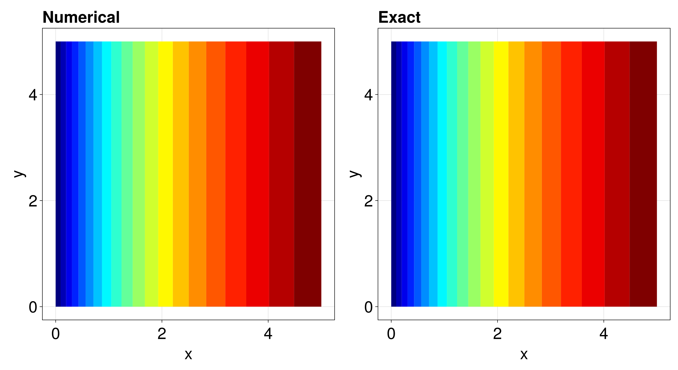

To finish, here is a benchmark comparing this problem to the corresponding SteadyFVMProblem.

initial_condition = zeros(DelaunayTriangulation.num_points(tri))
FVM.apply_dirichlet_conditions!(initial_condition, mesh, Conditions(mesh, BCs, InternalConditions())) # a good initial guess
fvm_prob = SteadyFVMProblem(FVMProblem(mesh, BCs;
    diffusion_function=(x, y, t, u, p) -> (x + 1) * (y + 2),
    final_time=Inf,
    initial_condition))

SteadyFVMProblem with 10000 nodes

using BenchmarkTools
@btime solve($prob, $KLUFactorization());

  15.368 ms (56 allocations: 17.12 MiB)

@btime solve($fvm_prob, $DynamicSS(TRBDF2(linsolve=KLUFactorization())));

  495.417 ms (223001 allocations: 114.30 MiB)

Just the code

An uncommented version of this example is given below. You can view the source code for this file here.

using FiniteVolumeMethod, SparseArrays, DelaunayTriangulation, LinearSolve
const FVM = FiniteVolumeMethod
function laplaces_equation(mesh::FVMGeometry,
    BCs::BoundaryConditions,
    ICs::InternalConditions=InternalConditions();
    diffusion_function=(x, y, p) -> 1.0,
    diffusion_parameters=nothing)
    conditions = Conditions(mesh, BCs, ICs)
    n = DelaunayTriangulation.num_points(mesh.triangulation)
    A = zeros(n, n)
    b = zeros(DelaunayTriangulation.num_points(mesh.triangulation))
    FVM.triangle_contributions!(A, mesh, conditions, diffusion_function, diffusion_parameters)
    FVM.boundary_edge_contributions!(A, b, mesh, conditions, diffusion_function, diffusion_parameters)
    FVM.apply_steady_dirichlet_conditions!(A, b, mesh, conditions)
    FVM.fix_missing_vertices!(A, b, mesh)
    Asp = sparse(A)
    prob = LinearProblem(Asp, b)
    return prob
end

using CairoMakie
lower_x = [1.0, 2.0]
lower_y = [0.0, 0.0]
θ = LinRange(0, π / 2, 100)
outer_arc_x = 2cos.(θ)
outer_arc_x[end] = 0.0 # must match with left_x
outer_arc_y = 2sin.(θ)
left_x = [0.0, 0.0]
left_y = [2.0, 1.0]
inner_arc_x = cos.(θ) |> reverse!
inner_arc_x[begin] = 0.0 # must match with left_x
inner_arc_y = sin.(θ) |> reverse!
boundary_x = [lower_x, outer_arc_x, left_x, inner_arc_x]
boundary_y = [lower_y, outer_arc_y, left_y, inner_arc_y]
boundary_nodes, points = convert_boundary_points_to_indices(boundary_x, boundary_y)
tri = triangulate(points; boundary_nodes)
refine!(tri; max_area=1e-3get_area(tri))
triplot(tri)

mesh = FVMGeometry(tri)

lower_f = (x, y, t, u, p) -> 0.0
outer_arc_f = (x, y, t, u, p) -> (π / 2 - atan(y, x)) * atan(y, x)
left_f = (x, y, t, u, p) -> 2x * y
inner_arc_f = (x, y, t, u, p) -> 2x * y
bc_f = (lower_f, outer_arc_f, left_f, inner_arc_f)
bc_types = (Dirichlet, Dirichlet, Dirichlet, Dirichlet)
BCs = BoundaryConditions(mesh, bc_f, bc_types)

prob = laplaces_equation(mesh, BCs, diffusion_function=(x, y, p) -> 1.0)

sol = solve(prob, KLUFactorization())

fig = Figure(fontsize=33)
ax = Axis(fig[1, 1], xlabel="x", ylabel="y", width=600, height=600)
tricontourf!(ax, tri, sol.u, levels=0:0.1:1, colormap=:jet)
resize_to_layout!(fig)
fig

initial_condition = zeros(DelaunayTriangulation.num_points(tri))
FVM.apply_dirichlet_conditions!(initial_condition, mesh, Conditions(mesh, BCs, InternalConditions())) # a good initial guess
fvm_prob = SteadyFVMProblem(FVMProblem(mesh, BCs;
    diffusion_function=(x, y, t, u, p) -> 1.0,
    initial_condition,
    final_time=Inf))

using SteadyStateDiffEq, OrdinaryDiffEq
fvm_sol = solve(fvm_prob, DynamicSS(TRBDF2()))

ax = Axis(fig[1, 2], xlabel="x", ylabel="y", width=600, height=600)
tricontourf!(ax, tri, fvm_sol.u, levels=0:0.1:1, colormap=:jet)
resize_to_layout!(fig)
fig

tri = triangulate_rectangle(0, 5, 0, 5, 100, 100, single_boundary=false)
mesh = FVMGeometry(tri)
zero_f = (x, y, t, u, p) -> 0.0
five_f = (x, y, t, u, p) -> 5.0
bc_f = (zero_f, five_f, zero_f, zero_f)
bc_types = (Neumann, Dirichlet, Neumann, Dirichlet) # bottom, right, top, left
BCs = BoundaryConditions(mesh, bc_f, bc_types)
diffusion_function = (x, y, p) -> (x + 1) * (y + 2)
prob = LaplacesEquation(mesh, BCs; diffusion_function)

sol = solve(prob, KLUFactorization())

fig = Figure(fontsize=33)
ax = Axis(fig[1, 1], xlabel="x", ylabel="y",
    width=600, height=600,
    title="Numerical", titlealign=:left)
tricontourf!(ax, tri, sol.u, levels=0:0.25:5, colormap=:jet)
ax = Axis(fig[1, 2], xlabel="x", ylabel="y",
    width=600, height=600,
    title="Exact", titlealign=:left)
u_exact = [5log(1 + x) / log(6) for (x, y) in DelaunayTriangulation.each_point(tri)]
tricontourf!(ax, tri, u_exact, levels=0:0.25:5, colormap=:jet)
resize_to_layout!(fig)
fig

initial_condition = zeros(DelaunayTriangulation.num_points(tri))
FVM.apply_dirichlet_conditions!(initial_condition, mesh, Conditions(mesh, BCs, InternalConditions())) # a good initial guess
fvm_prob = SteadyFVMProblem(FVMProblem(mesh, BCs;
    diffusion_function=(x, y, t, u, p) -> (x + 1) * (y + 2),
    final_time=Inf,
    initial_condition))

This page was generated using Literate.jl.

1See, for example, this paper by Rangogni and Occhi (1987).
2This problem comes from here.
3This is the first example from this paper by Rangogni and Occhi (1987).