Helmholtz Equation with Inhomogeneous Boundary Conditions

In this tutorial, we consider the following steady state problem:

\[\begin{equation} \begin{aligned} \grad^2 u(\vb x) + u(\vb x) &= 0 & \vb x \in [-1, 1]^2 \\ \pdv{u}{\vb n} &= 1 & \vb x \in\partial[-1,1]^2. \end{aligned} \end{equation}\]

We can define this problem in the same way we have defined previous problems, except that the final FVMProblem must be wrapped in a SteadyFVMProblem. Let us start by defining the mesh and the boundary conditions.

using DelaunayTriangulation, FiniteVolumeMethod
tri = triangulate_rectangle(-1, 1, -1, 1, 125, 125, single_boundary=true)
mesh = FVMGeometry(tri)

FVMGeometry with 15625 control volumes, 30752 triangles, and 46376 edges

For the boundary condition,

\[\pdv{u}{\vb n} = 1,\]

which is the same as $\grad u \vdot \vu n = 1$, this needs to be expressed in terms of $\vb q$. Since $\vb q = -\grad u$ for this problem, the boundary condition is $\vb q \vdot \vu n = -1$.

BCs = BoundaryConditions(mesh, (x, y, t, u, p) -> -one(u), Neumann)

BoundaryConditions with 1 boundary condition with type Neumann

To now define the problem, we note that the initial_condition and final_time fields have different interpretations for steady state problems. The initial_condition now serves as an initial estimate for the steady state solution, which is needed for the nonlinear solver, and final_time should now be Inf. For the initial condition, let us simply let the initial estimate be all zeros. For the diffusion and source terms, note that previously we have been considered equations of the form

\[\pdv{u}{t} + \div\vb q = S \quad \textnormal{or} \quad \pdv{u}{t} = \div[D\grad u] + S,\]

while steady state problems take the form

\[\div\vb q = S \quad \textnormal{or} \quad \div[D\grad u] + S = 0.\]

So, for this problem, $D = 1$ and $S = u$.

diffusion_function = (x, y, t, u, p) -> one(u)
source_function = (x, y, t, u, p) -> u
initial_condition = zeros(DelaunayTriangulation.num_solid_vertices(tri))
final_time = Inf
prob = FVMProblem(mesh, BCs;
    diffusion_function,
    source_function,
    initial_condition,
    final_time)

FVMProblem with 15625 nodes and time span (0.0, Inf)

steady_prob = SteadyFVMProblem(prob)

SteadyFVMProblem with 15625 nodes

To now solve this problem, we use a Newton-Raphson solver. Alternative solvers, such as DynamicSS(TRBDF2(linsolve=KLUFactorization()), reltol=1e-4) from SteadyStateDiffEq can also be used. A good method could be to use a simple solver, like NewtonRaphson(), and then use that solution as the initial guess in a finer algorithm like the DynamicSS algorithm above.

using NonlinearSolve
sol = solve(steady_prob, NewtonRaphson())
copyto!(prob.initial_condition, sol.u) # this also changes steady_prob's initial condition
using SteadyStateDiffEq, LinearSolve, OrdinaryDiffEq
sol = solve(steady_prob, DynamicSS(TRBDF2(linsolve=KLUFactorization())))

retcode: Success
u: 15625-element Vector{Float64}:
 -1.284086882618605
 -1.3001602399337973
 -1.3160471807169647
 -1.3317536108619856
 -1.347278372873141
  ⋮
 -1.3472783728731401
 -1.3317536108619847
 -1.3160471807169638
 -1.3001602399337964
 -1.284086882618604

For this problem, this correction by DynamicSS doesn't seem to actually be needed. Now let's visualise.

using CairoMakie
fig, ax, sc = tricontourf(tri, sol.u, levels=-2.5:0.15:-1.0, colormap=:matter)
fig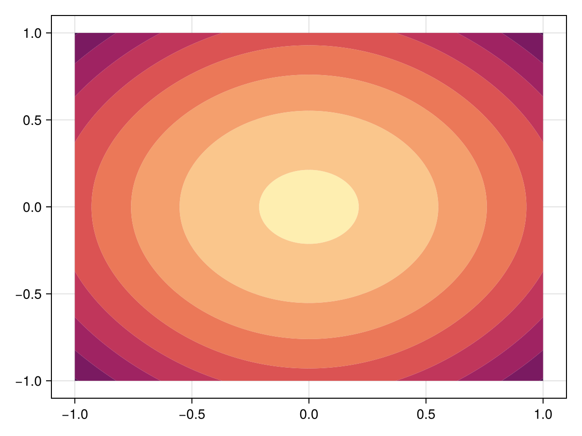

Just the code

An uncommented version of this example is given below. You can view the source code for this file here.

using DelaunayTriangulation, FiniteVolumeMethod
tri = triangulate_rectangle(-1, 1, -1, 1, 125, 125, single_boundary=true)
mesh = FVMGeometry(tri)

BCs = BoundaryConditions(mesh, (x, y, t, u, p) -> -one(u), Neumann)

diffusion_function = (x, y, t, u, p) -> one(u)
source_function = (x, y, t, u, p) -> u
initial_condition = zeros(DelaunayTriangulation.num_solid_vertices(tri))
final_time = Inf
prob = FVMProblem(mesh, BCs;
    diffusion_function,
    source_function,
    initial_condition,
    final_time)

steady_prob = SteadyFVMProblem(prob)

using NonlinearSolve
sol = solve(steady_prob, NewtonRaphson())
copyto!(prob.initial_condition, sol.u) # this also changes steady_prob's initial condition
using SteadyStateDiffEq, LinearSolve, OrdinaryDiffEq
sol = solve(steady_prob, DynamicSS(TRBDF2(linsolve=KLUFactorization())))

using CairoMakie
fig, ax, sc = tricontourf(tri, sol.u, levels=-2.5:0.15:-1.0, colormap=:matter)
fig

This page was generated using Literate.jl.