Laplace's Equation with Internal Dirichlet Conditions

In this tutorial, we consider Laplace's equation with some additional complexity put into the problem via internal Dirichlet conditions:

\[\begin{equation} \begin{aligned} \grad^2 u &= 0 & \vb x \in [0, 1]^2, \\ u(0, y) &= 100y & 0 \leq y \leq 1, \\ u(1, y) &= 100y & 0 \leq y \leq 1, \\ u(x, 0) &= 0 & 0 \leq x \leq 1, \\ u(x, 1) &= 100 & 0 \leq x \leq 1, \\ u(1/2, y) &= 0 & 0 \leq y \leq 2/5. \end{aligned} \end{equation}\]

To start with solving this problem, let us define an initial mesh.

using DelaunayTriangulation, FiniteVolumeMethod
tri = triangulate_rectangle(0, 1, 0, 1, 50, 50, single_boundary=false)

Delaunay Triangulation.
   Number of vertices: 2500
   Number of triangles: 4802
   Number of edges: 7301
   Has boundary nodes: true
   Has ghost triangles: true
   Curve-bounded: false
   Weighted: false
   Constrained: true

In this mesh, we don't have any points that lie exactly on the line $\{x = 1/2, 0 \leq y \leq 2/5\}$, so we cannot enforce this constraint exactly.^[1] Instead, we need to add these points into tri. We do not need to add any constrained edges in this case, since these internal conditions are enforced only at points.

Let us now add in the points.

using CairoMakie
new_points = LinRange(0, 2 / 5, 250)
for y in new_points
    add_point!(tri, 1 / 2, y)
end
fig, ax, sc = triplot(tri)
fig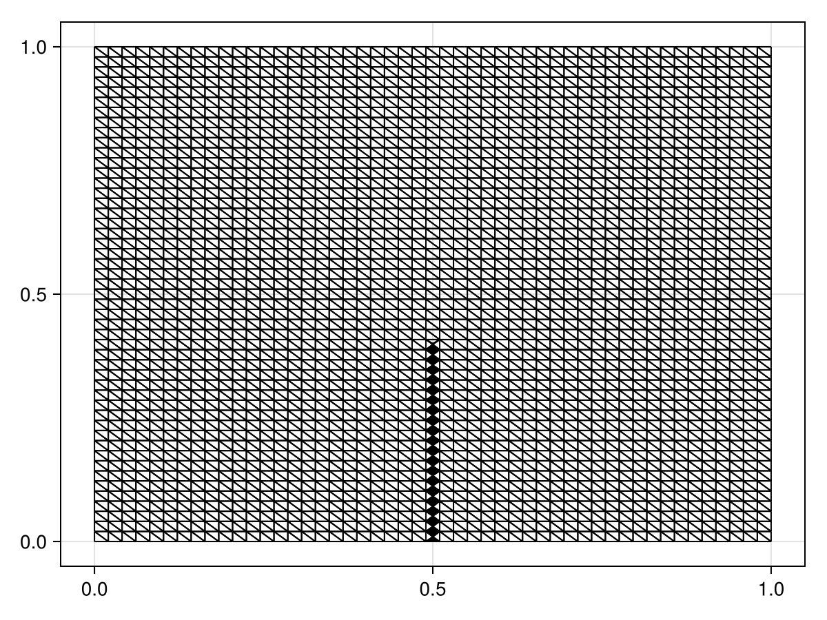

It may also help to refine the mesh slightly.

refine!(tri, max_area=1e-4)
fig, ax, sc = triplot(tri)
fig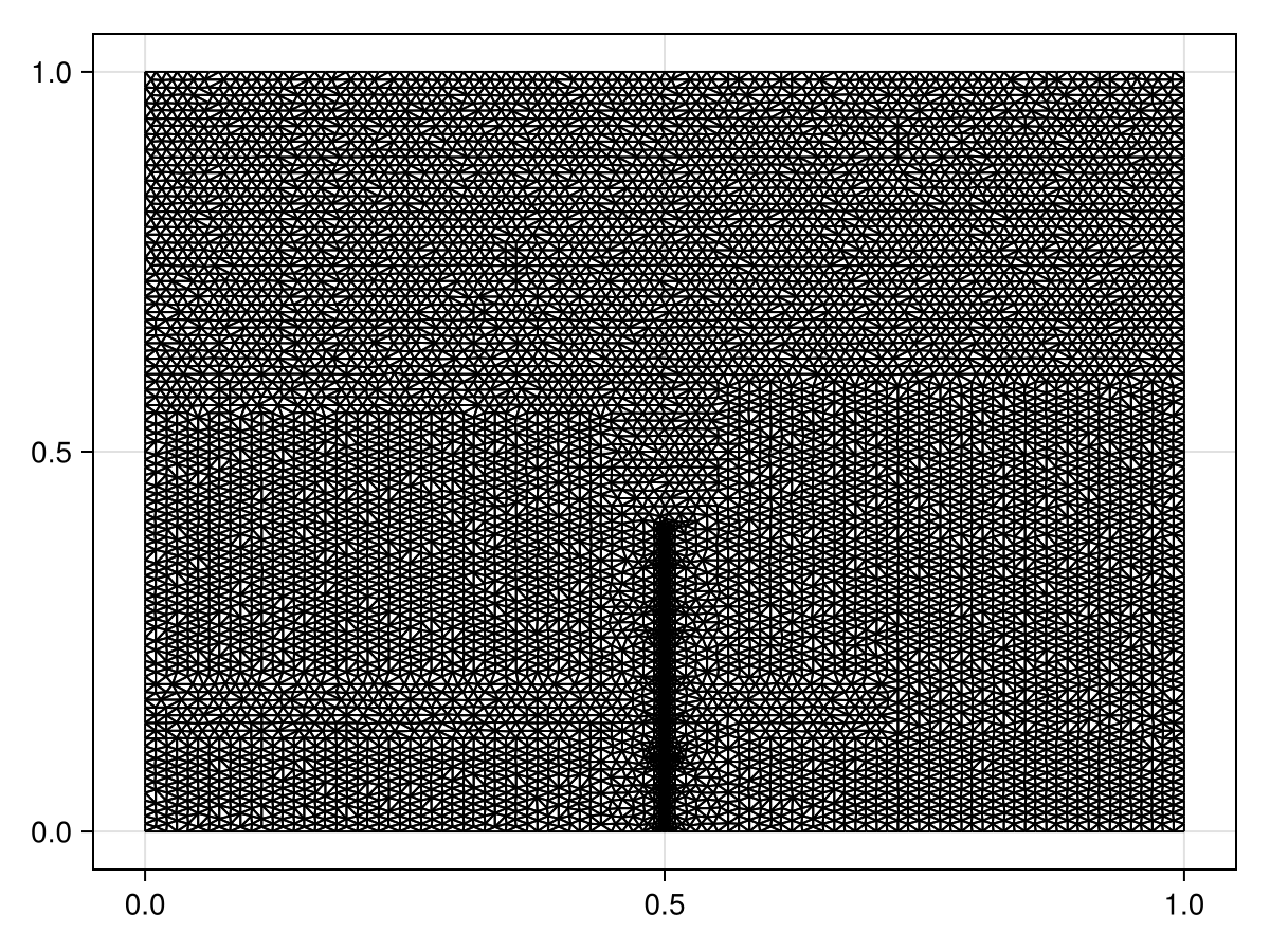

mesh = FVMGeometry(tri)

FVMGeometry with 10192 control volumes, 20006 triangles, and 30197 edges

Now that we have the mesh, we can define the boundary conditions. Remember that the order of the boundary indices is the bottom wall, right wall, top wall, and then the left wall.

bc_bot = (x, y, t, u, p) -> zero(u)
bc_right = (x, y, t, u, p) -> oftype(u, 100y) # helpful to have each bc return the same type
bc_top = (x, y, t, u, p) -> oftype(u, 100)
bc_left = (x, y, t, u, p) -> oftype(u, 100y)
bcs = (bc_bot, bc_right, bc_top, bc_left)
types = (Dirichlet, Dirichlet, Dirichlet, Dirichlet)
BCs = BoundaryConditions(mesh, bcs, types)

BoundaryConditions with 4 boundary conditions with types (Dirichlet, Dirichlet, Dirichlet, Dirichlet)

We now need to define the internal conditions. This is done using InternalConditions. First, we need to find all the vertices that lie on the line $\{x = 1/2, 0 \leq y \leq 2/5\}$. We could compute these manually, but let's find them programatically instead for the sake of demonstration.

function find_all_points_on_line(tri)
    vertices = Int[]
    for i in each_solid_vertex(tri)
        x, y = get_point(tri, i)
        if x == 1 / 2 && 0 ≤ y ≤ 2 / 5
            push!(vertices, i)
        end
    end
    return vertices
end
vertices = find_all_points_on_line(tri)
fig, ax, sc = triplot(tri)
points = [get_point(tri, i) for i in vertices]
scatter!(ax, points, color=:red, markersize=10)
fig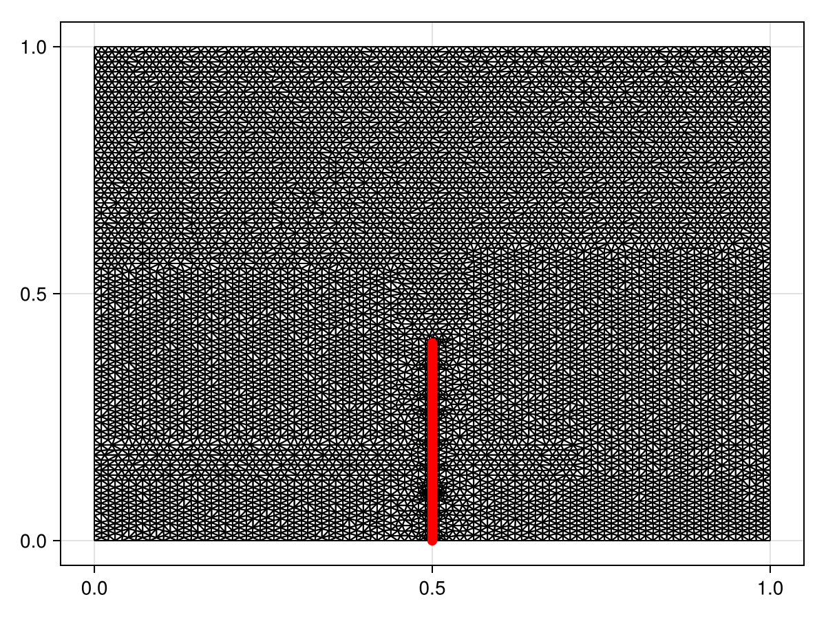

Now that we have the vertices, we can define the internal conditions. We need to provide InternalConditions with a Dict that maps each vertex in vertices to a function index that corresponds to the condition for that vertex. In this case, that function index is 1 as we only have a single function.

ICs = InternalConditions((x, y, t, u, p) -> zero(u),
    dirichlet_nodes=Dict(vertices .=> 1))

InternalConditions with 250 Dirichlet nodes and 0 Dudt nodes

Now we can define the problem. As discussed in the Helmholtz tutorial, we are looking to define a steady state problem, and so the initial condition needs to be a suitable initial guess of what the solution could be. Looking to the boundary and internal conditions, one suitable guess is $u(x, y) = 100y$ with $u(1/2, y) = 0$ for $0 \leq y \leq 2/5$; in fact, $u(x, y) = 100y$ is the solution of the problem without the internal condition. Let us now use this to define our initial condition.

initial_condition = zeros(DelaunayTriangulation.num_points(tri))
for i in each_solid_vertex(tri)
    x, y = get_point(tri, i)
    initial_condition[i] = ifelse(x == 1 / 2 && 0 ≤ y ≤ 2 / 5, 0, 100y)
end

Now let's define the problem. The internal conditions are provided as the third argument of FVMProblem.

diffusion_function = (x, y, t, u, p) -> one(u) # ∇²u = ∇⋅[D∇u], D = 1
final_time = Inf
prob = FVMProblem(mesh, BCs, ICs;
    diffusion_function,
    initial_condition,
    final_time)

FVMProblem with 10192 nodes and time span (0.0, Inf)

steady_prob = SteadyFVMProblem(prob)

SteadyFVMProblem with 10192 nodes

Now let's solve the problem.

using SteadyStateDiffEq, LinearSolve, OrdinaryDiffEq
sol = solve(steady_prob, DynamicSS(TRBDF2(linsolve=KLUFactorization())))

retcode: Success
u: 10195-element Vector{Float64}:
  0.0
  0.0
  0.0
  0.0
  0.0
  ⋮
  0.0
  0.0
 84.62249591879079
  7.598201538967747
  0.0

fig, ax, sc = tricontourf(tri, sol.u, levels=LinRange(0, 100, 28))
tightlimits!(ax)
fig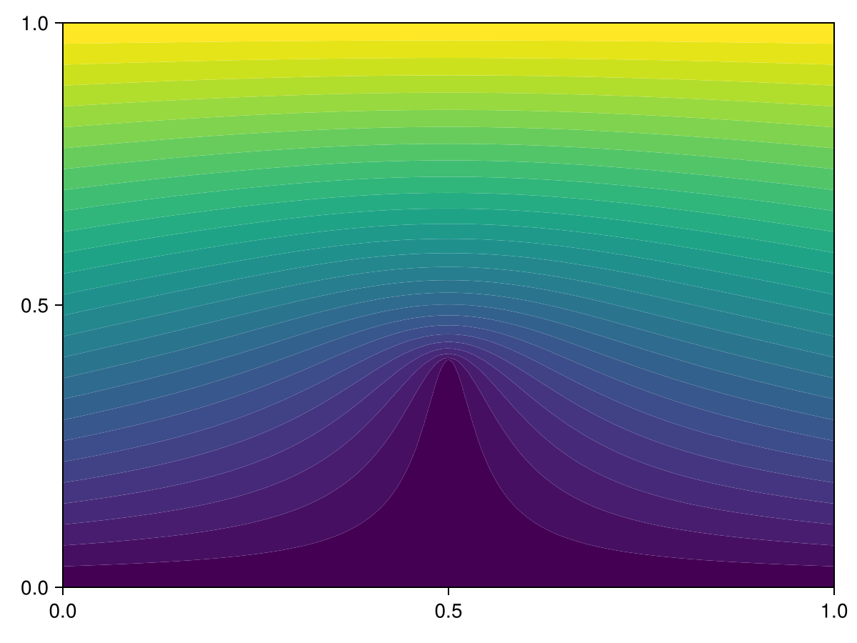

Just the code

An uncommented version of this example is given below. You can view the source code for this file here.

using DelaunayTriangulation, FiniteVolumeMethod
tri = triangulate_rectangle(0, 1, 0, 1, 50, 50, single_boundary=false)

using CairoMakie
new_points = LinRange(0, 2 / 5, 250)
for y in new_points
    add_point!(tri, 1 / 2, y)
end
fig, ax, sc = triplot(tri)
fig

refine!(tri, max_area=1e-4)
fig, ax, sc = triplot(tri)
fig

mesh = FVMGeometry(tri)

bc_bot = (x, y, t, u, p) -> zero(u)
bc_right = (x, y, t, u, p) -> oftype(u, 100y) # helpful to have each bc return the same type
bc_top = (x, y, t, u, p) -> oftype(u, 100)
bc_left = (x, y, t, u, p) -> oftype(u, 100y)
bcs = (bc_bot, bc_right, bc_top, bc_left)
types = (Dirichlet, Dirichlet, Dirichlet, Dirichlet)
BCs = BoundaryConditions(mesh, bcs, types)

function find_all_points_on_line(tri)
    vertices = Int[]
    for i in each_solid_vertex(tri)
        x, y = get_point(tri, i)
        if x == 1 / 2 && 0 ≤ y ≤ 2 / 5
            push!(vertices, i)
        end
    end
    return vertices
end
vertices = find_all_points_on_line(tri)
fig, ax, sc = triplot(tri)
points = [get_point(tri, i) for i in vertices]
scatter!(ax, points, color=:red, markersize=10)
fig

ICs = InternalConditions((x, y, t, u, p) -> zero(u),
    dirichlet_nodes=Dict(vertices .=> 1))

initial_condition = zeros(DelaunayTriangulation.num_points(tri))
for i in each_solid_vertex(tri)
    x, y = get_point(tri, i)
    initial_condition[i] = ifelse(x == 1 / 2 && 0 ≤ y ≤ 2 / 5, 0, 100y)
end

diffusion_function = (x, y, t, u, p) -> one(u) # ∇²u = ∇⋅[D∇u], D = 1
final_time = Inf
prob = FVMProblem(mesh, BCs, ICs;
    diffusion_function,
    initial_condition,
    final_time)

steady_prob = SteadyFVMProblem(prob)

using SteadyStateDiffEq, LinearSolve, OrdinaryDiffEq
sol = solve(steady_prob, DynamicSS(TRBDF2(linsolve=KLUFactorization())))

fig, ax, sc = tricontourf(tri, sol.u, levels=LinRange(0, 100, 28))
tightlimits!(ax)
fig

This page was generated using Literate.jl.